Decision Trees for Classification - Example
- 5 minutes read - 950 wordsIntroduction
Decision Trees are a powerful, yet simple Machine Learning Model. An advantage of their simplicity is that we can build and understand them step by step. In this post, we are looking at a simplified example to build an entire Decision Tree by hand for a classification task. After calculating the tree, we will use the sklearn package and compare the results. To learn how to build a Decision Tree for a regression problem, please refer to the article Decision Trees for Regression - Example. For a general introduction to Decision Trees and how to build them please check the article Decision Trees - Explained.
Data
The Dataset we use in this post contains only 10 samples. We want to decide whether a person should go rock climbing or not, depending on whether they like height, like goats, and their age. That is the dataset contains three input features, of which two are categorical, as both have exactly two classes they are even binary and one is numerical. The target variable is also categorical.
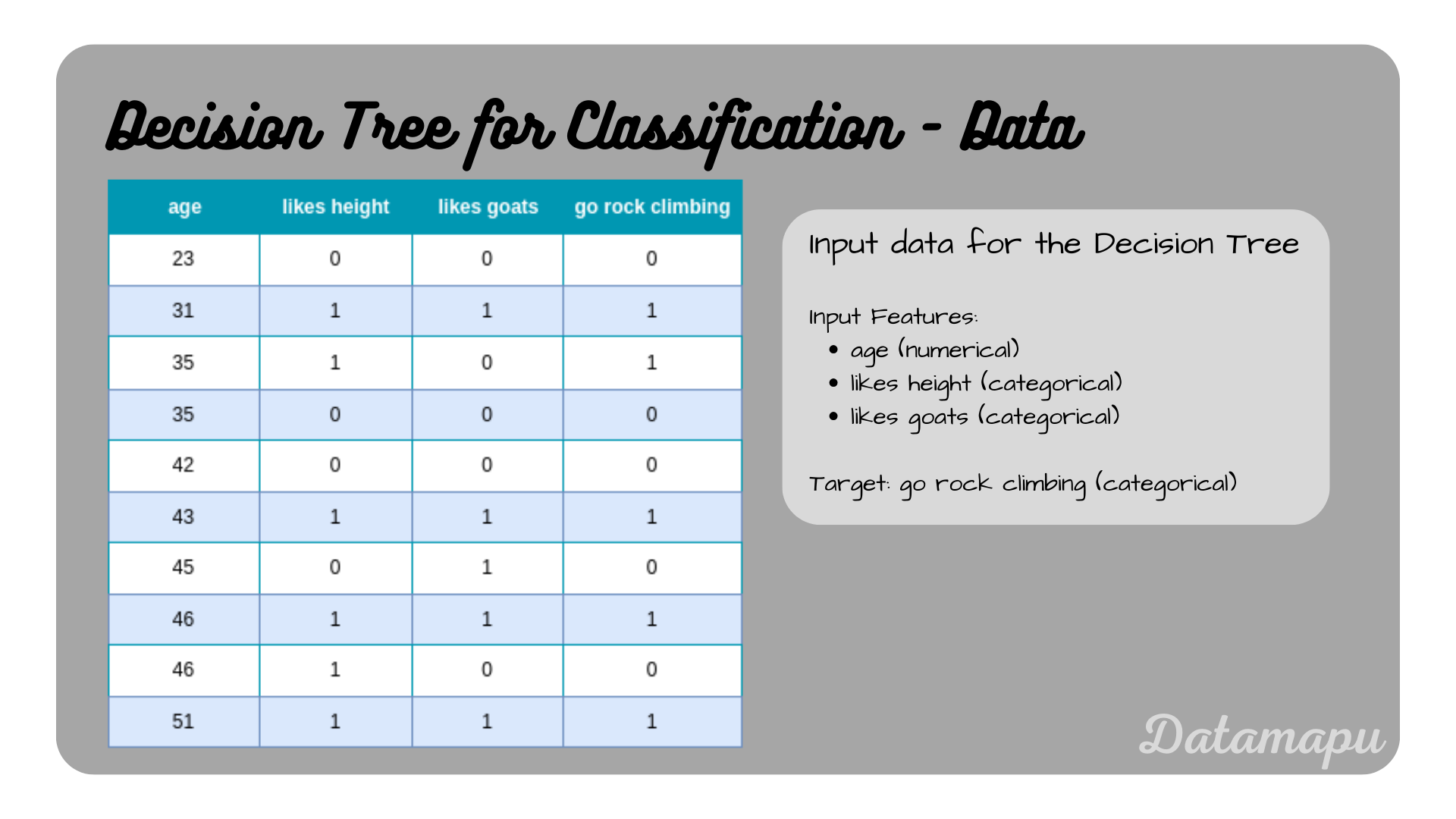 Data used to build a Decision Tree.
Build the Tree
Our target data is categorical, that is we are building a Decision Tree for a classification problem. The main step in building a Decision Tree is splitting the data according to a splitting criterion. There exist different splitting criteria. We will use the Gini Impurity, which is the most common criterion and also used in the sklearn package as the default criterion. The Gini Impurity for a Dataset $D$ that is split into two Datasets $D_1$ and $D_2$, is defined as
$$Gini(D) = \frac{n_1}{n} \cdot Gini(D_1) + \frac{n_2}{n} \cdot Gini(D_2),$$
with $n = n_1 + n_2$ the size of the dataset $D$, its subsets $D_1$, $D_2$, and
$$Gini(D_i) = 1 - \sum_{j=1}^c p_j^2.$$
With $p_j$ being the probability that a randomly drawn sample from this node belongs to class $j$ and $c$ the number of classes. Starting with the root node, which contains the entire dataset to make the first split, we calculate the Gini Impurity for all three features in the dataset (‘age’, ’likes goats’, and ’likes height’) and then choose the feature that gives the lowest Gini Impurity. We will start with the categorical features.
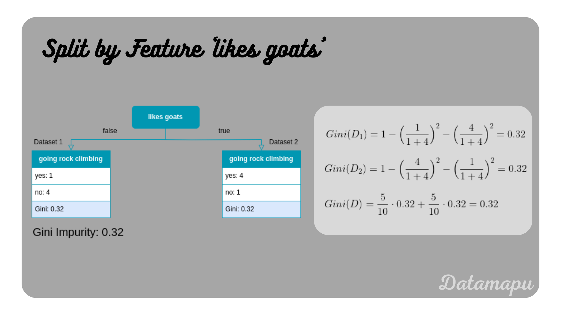 Gini Impurity if the split is done with the feature ’likes goats’.
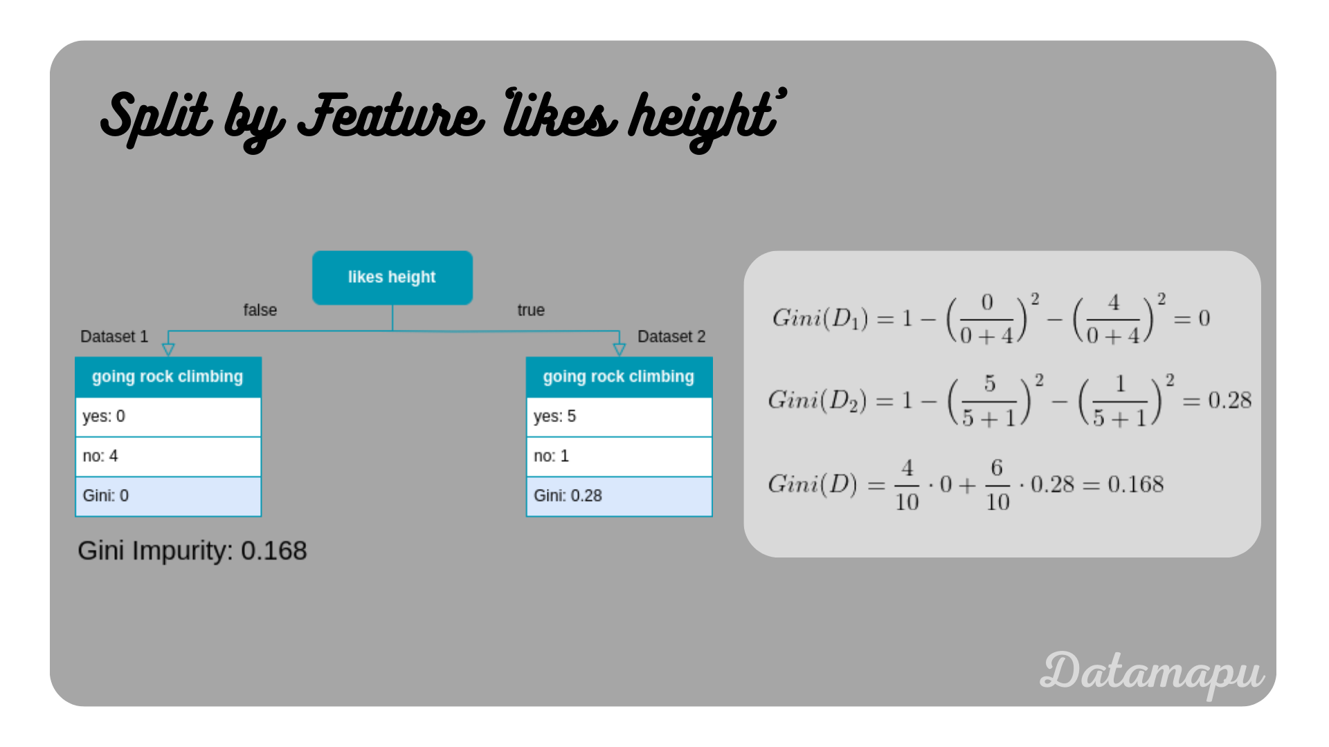 Gini Impurity if the split is done with the feature ’likes height’.
From these two features, we can see that ’likes height’ has a lower Gini Impurity and would therefore be preferred to ’likes goats’. For numerical features, the calculation is a bit more complex. The strategy is the following
- Order the numerical feature in an ascending way.
- Calculate the mean of neighboring items. These are all possible splits.
- Determine the Gini Impurity for all possible splits.
- Choose the lowest of these Gini Impurities as the Gini Impurity of this feature.
For the feature ‘age’ the values are already ordered, but we still need to calculate the means to find all possible splits.
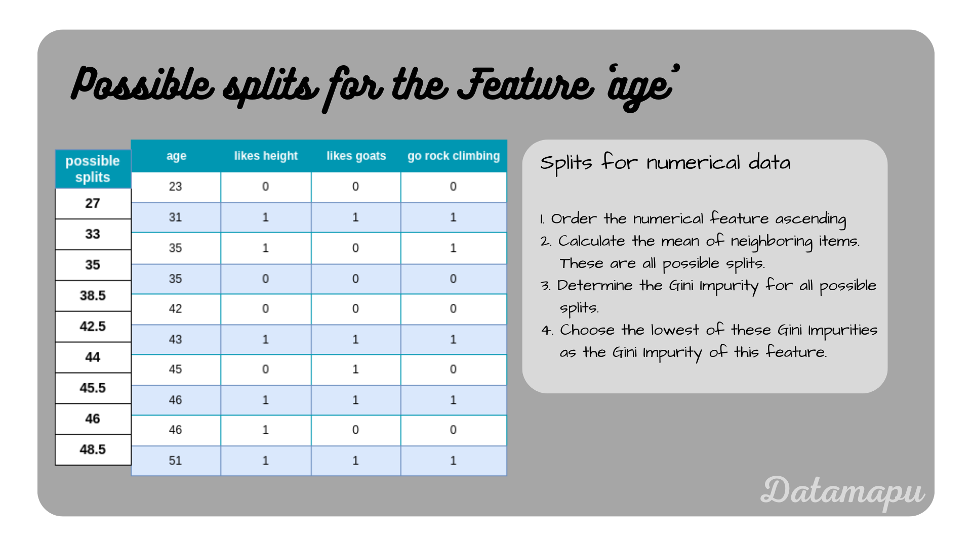 Possible splits for the numerical feature ‘age’.
Now, let’s calculate the Gini Impurity for each of these splits.
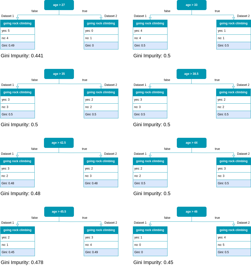 All possible splits for ‘age’ and their corresponding Gini Impurity.
From the above calculations, we see that all Gini Impurities for the feature ‘age’ are higher than the one for ’likes height’, which was our previous best feature. That is ’likes height’ is the feature that results in the lowest Gini Impurity of all three features and we will use it for the first split of the tree.
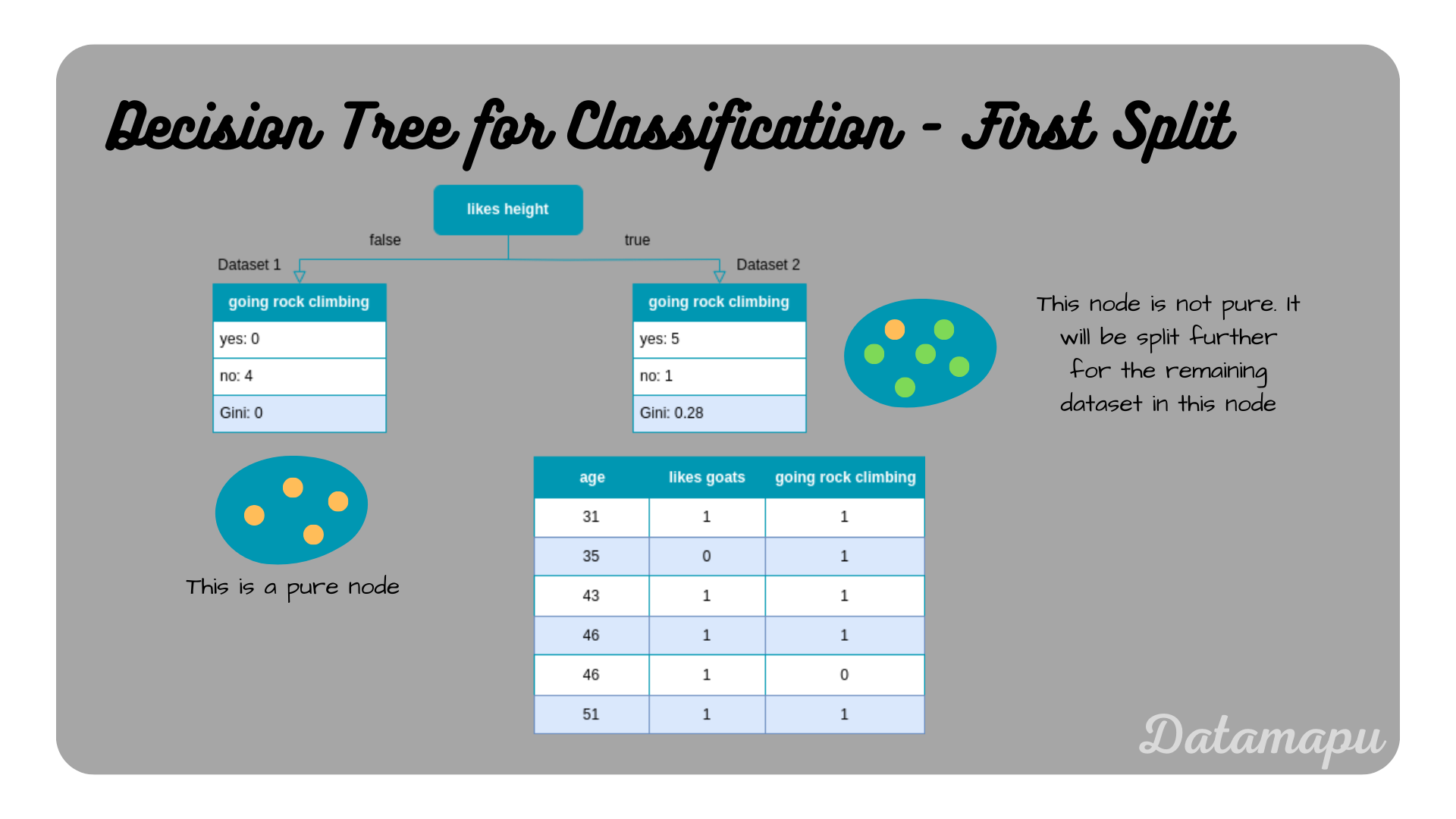 First split of the Decision Tree.
After this first split, one of the resulting nodes is already pure, that is no further split is possible and we have the first leaf of our tree. The second node is not pure and will be split using the remaining dataset. We calculate the Gini Impurity for the features ’likes goats’ and ‘age’ exactly as we did for the entire dataset.
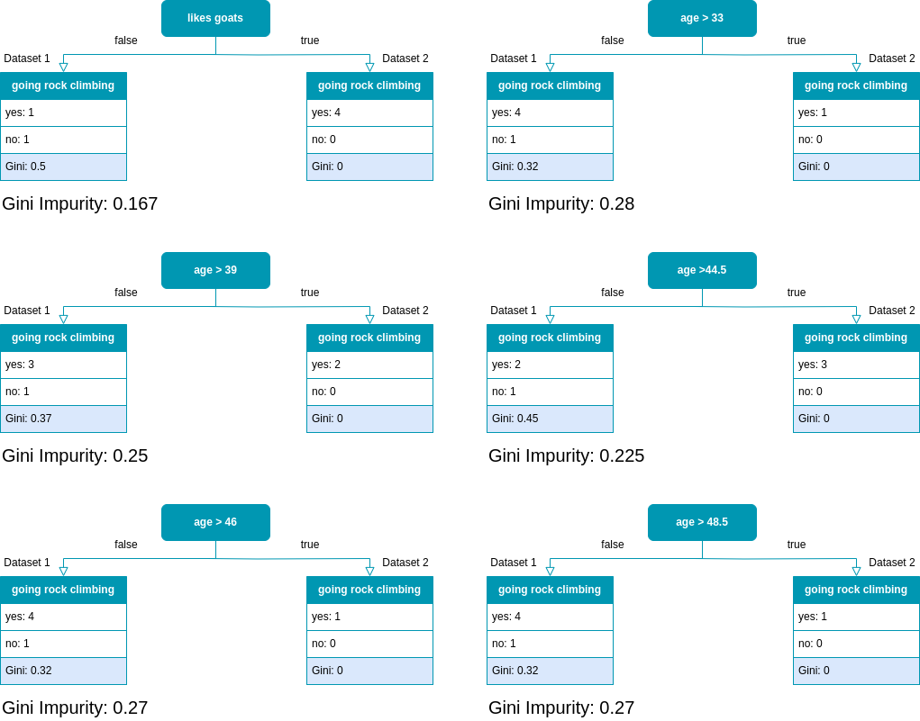 All possible splits for the second split.
From the above plot we see that the feature with the lowest Gini Impurity is ’likes goats’. This will thus be our second split.
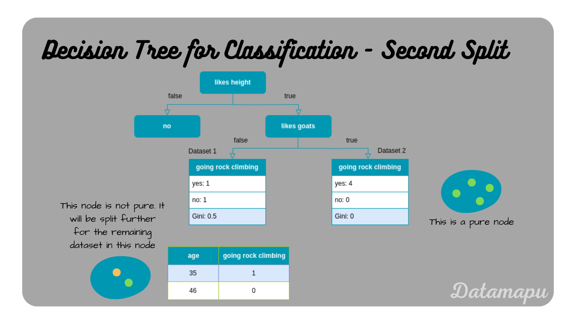 Second split of the Decision Tree.
Now there is just one node remaining that we need to split. The final Decision Tree has the following form.
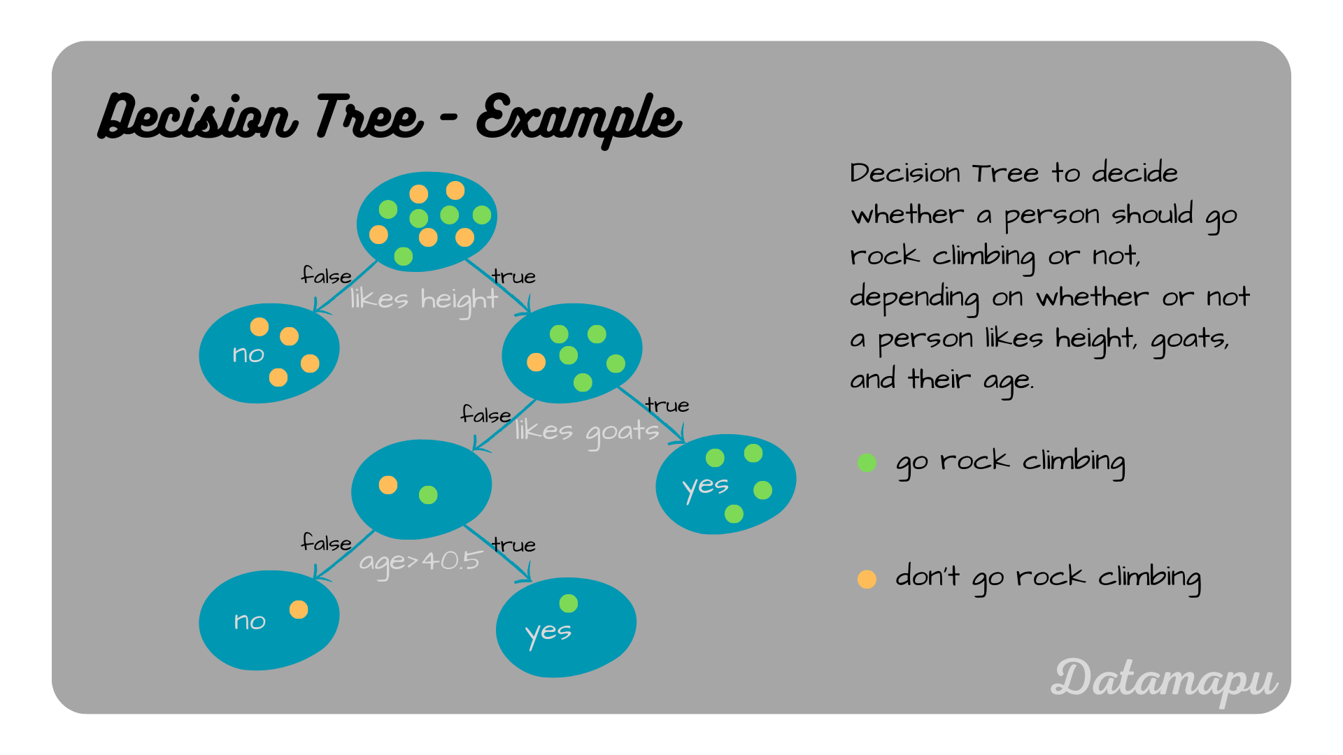 Illustration of the final Decision Tree.
Fit a Model in Python
In Python we can use sklearn to fit a Decision Tree. For a classification task, we use the DecisionTreeClassifier Class.
| |
We can visualize the fitted tree also using sklearn. Note, that there are some slight differences in the notations, but the tree build using sklearn is exactly the same we build by calculating the splits by hand.
| |
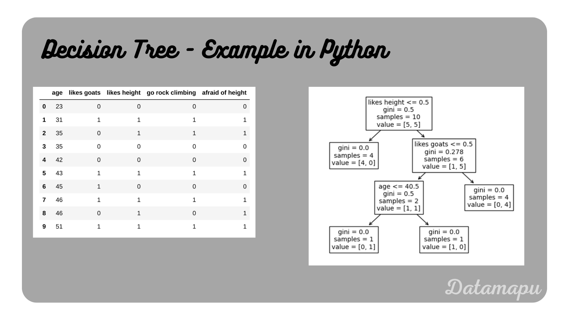 Illustration of the final Decision Tree built in Python.
Summary
In this article, we analyzed in detail how to build a Decision Tree for a classification task, especially how to choose the best split step by step. A more realistic example of how to fit a Decision Tree to a dataset using sklearn can be found on kaggle.
If this blog is useful for you, please consider supporting.
