Decision Trees for Regression - Example

Introduction

A Decision Tree is a simple Machine Learning model that can be used for both regression and classification tasks. In the article Decision Trees for Classification - Example a Decision Tree for a classification problem is developed in detail. In this post, we consider a regression problem and build a Decision Tree step by step for a simplified dataset. Additionally, we use sklearn to fit a model to the data and compare the results. To learn about Decision Trees in a more general setup, please refer to Decision Trees - Explained

Data

We use a dataset that contains only 10 samples. We are predicting the number of meters climbed by a person, depending on their age, whether they like goats, and whether they like height. That is we have three input features of which one is numerical and two are categorical. The two categorical features consist of two classes each and are therefore binary. The target variable is numerical.

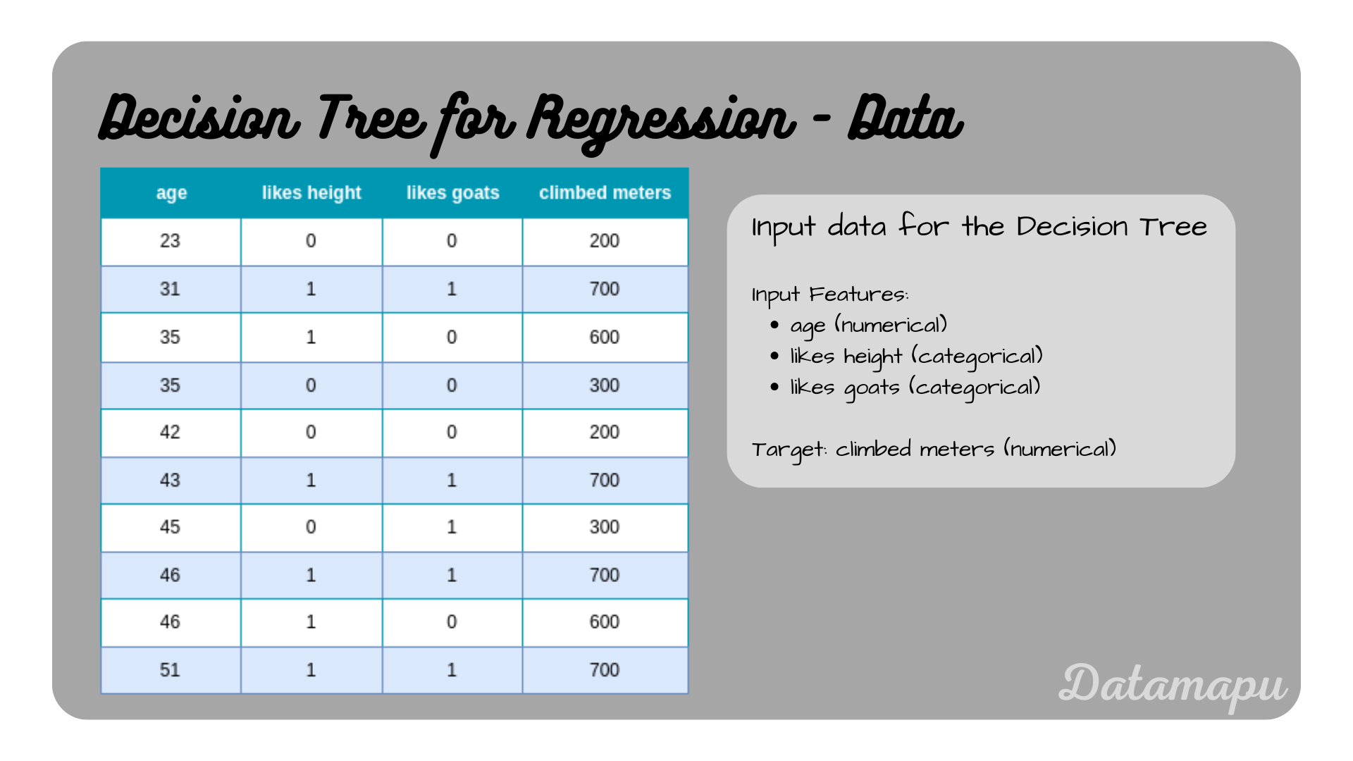Data used to build a Decision Tree.

Build the Tree

The essential part of building a Decision Tree is finding the best split of the data to grow the tree. The split is done by a certain criterion, which depends on whether the target data is numerical or categorical. In this example, we use the Sum of Squared Errors (SSE), which is also the default choice in the sklearn framework. The SSE for a dataset $D$, that is split into two subsets $D_1$ and $D_2$ is defined as

$$SSE(D) = SSE(D_1) + SSE(D_2),$$

with

$$SSE(D_i) = \frac{1}{n_i}\sum_{j=1}^{n_i}(x_j-\bar{x}_i)^2,$$

and $x_i, \dots, x_{n_i}$ the items of $D_i$. We calculate the SSE for all three features and the feature with the lowest SSE is then chosen for the first split. We start with the two categorical features.

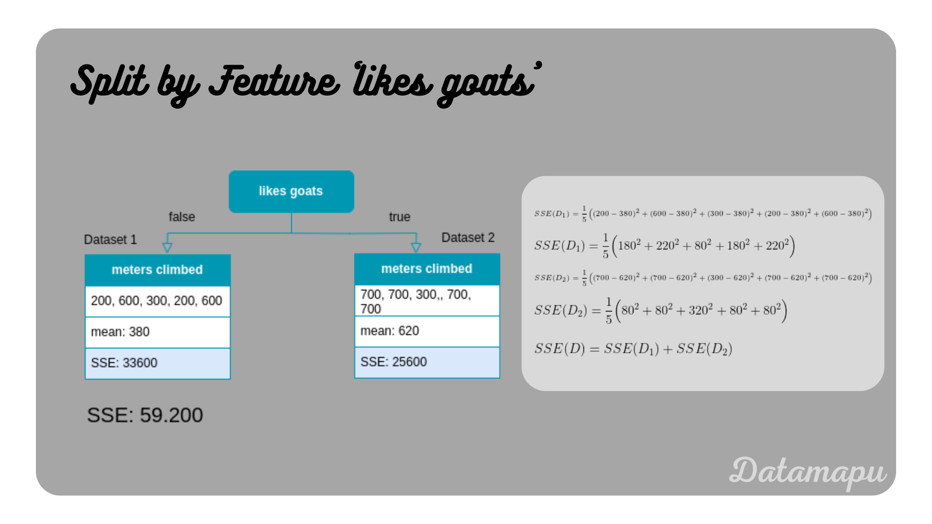SSE for spliting the tree using the feature ’likes goats’.

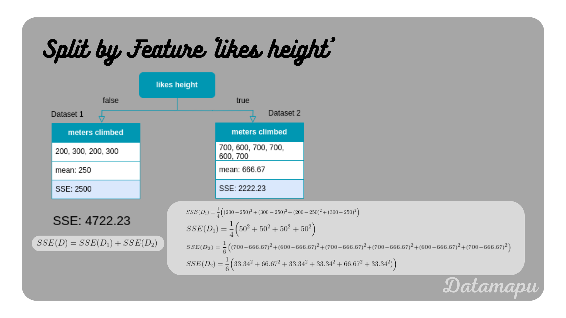SSE for spliting the tree using the feature ’likes height’.

From these two features, we see that ’likes height’ has a lower SSE than ’likes goats’, that is ’likes height’ would be preferred compared to ’likes goat’. For numerical features, the procedure is similar but takes more calculations. For the feature ‘age’ we proceed with the following step

1. Order the numerical feature in an ascending way.
2. Calculate the mean of neighboring items. These are all possible splits.
3. Determine the SSE for all possible splits.
4. Choose the lowest of these SSEs as the SSE of this feature.

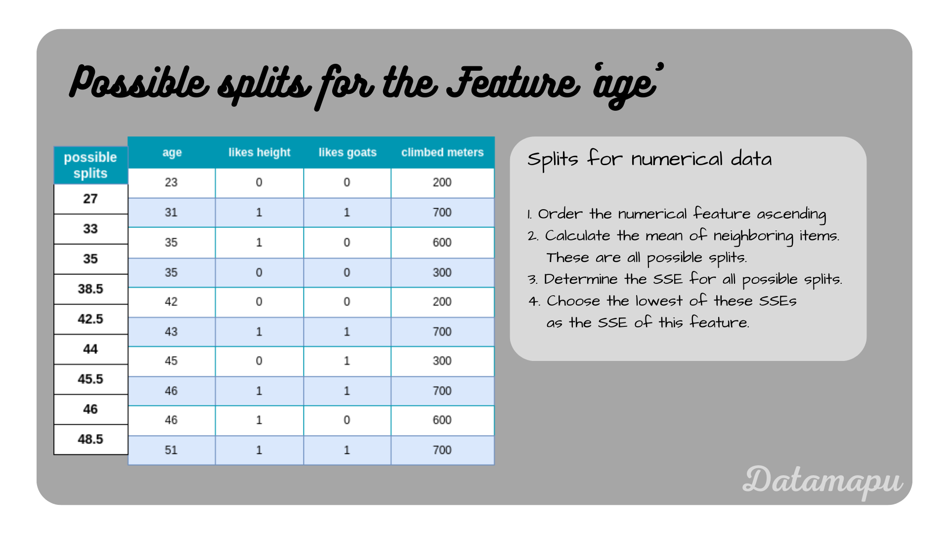Possible splits for the numerical feature ‘age’.

Now, let’s calculate the SSE for each of these splits.

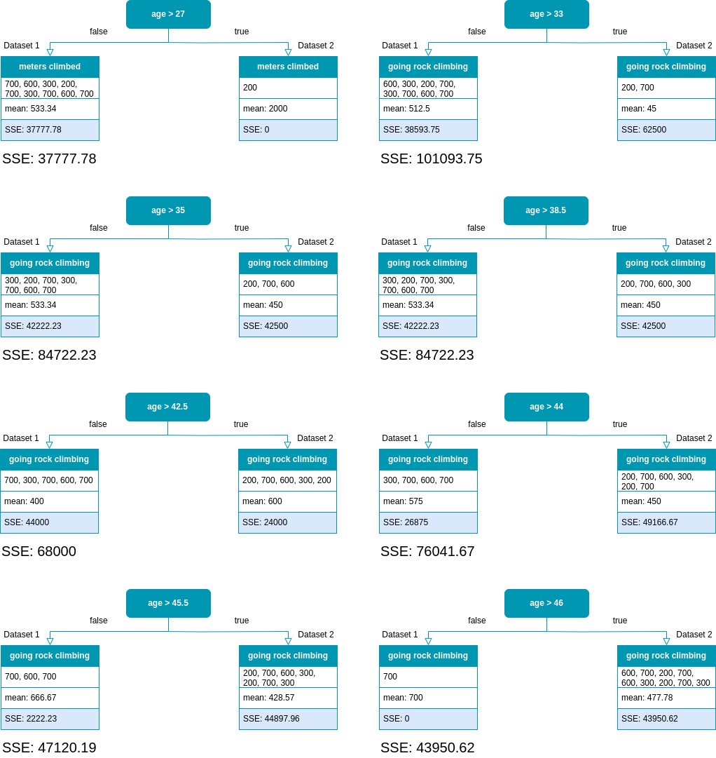Possible splits for the numerical feature ‘age’ and their corresponding SSE.

From the above results, we see that all SSE values for the feature ‘age’ are higher than the one for ’likes height’, which was the previous best feature. Therefore ’likes height’ remains the best feature to split the data and we can build the first level of our tree.

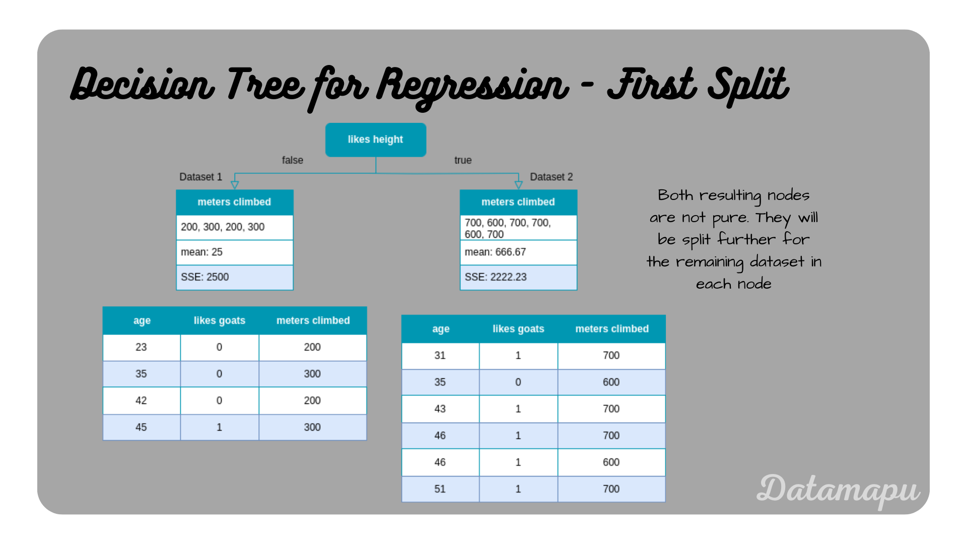First split of the tree using the feature ’likes height’.

Both nodes resulting from this split are not pure and are split further. We start with the left-hand side. The procedure is the same as for the entire dataset. We have two features remaining ’likes goats’ and ‘age’. The following plot shows the remaining two datasets with all possible splits along the feature ‘age’.

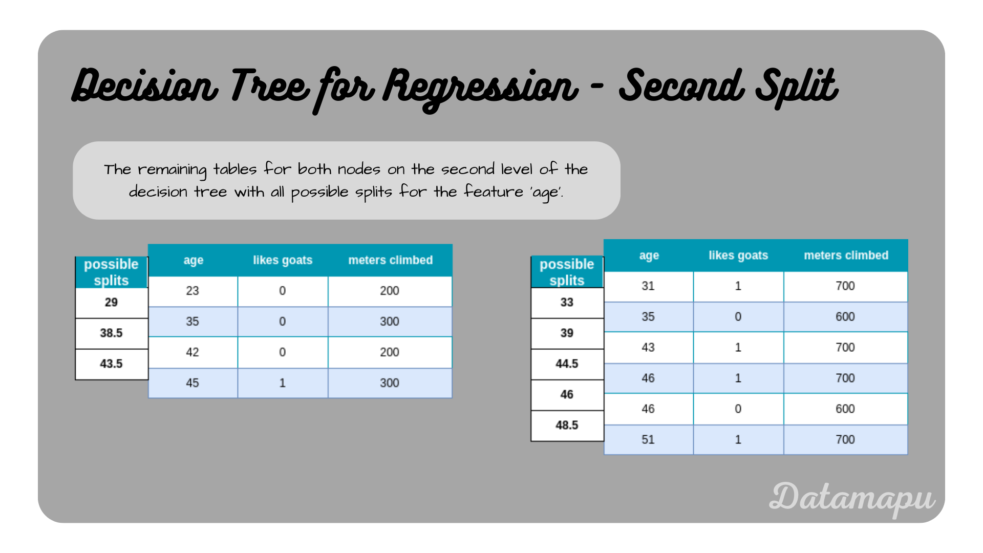The two datasets remaining for further splitting.

We start with the left-hand side and calculate the SSE for all possible splits.

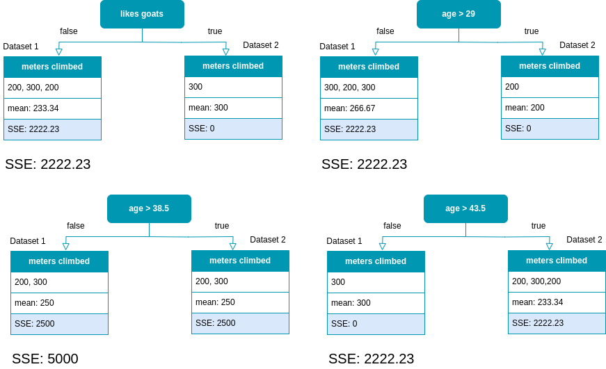All possible splits for the first dataset of the second split.

The results show, that several splits lead to the same SSE. This means we could choose any of them, for the next split. We use the feature ’likes goats’. Now, we do the same for the right-hand side of the tree.

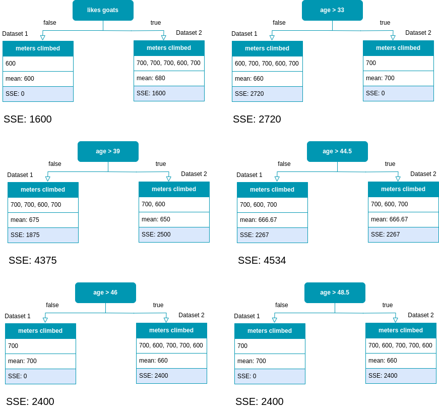All possible splits for the second dataset of the second split.

We can see, that the feature ’likes goats’ results in the lowest SSE. That is we will choose this feature for the next split. We now have constructed the second level of our Decision Tree.

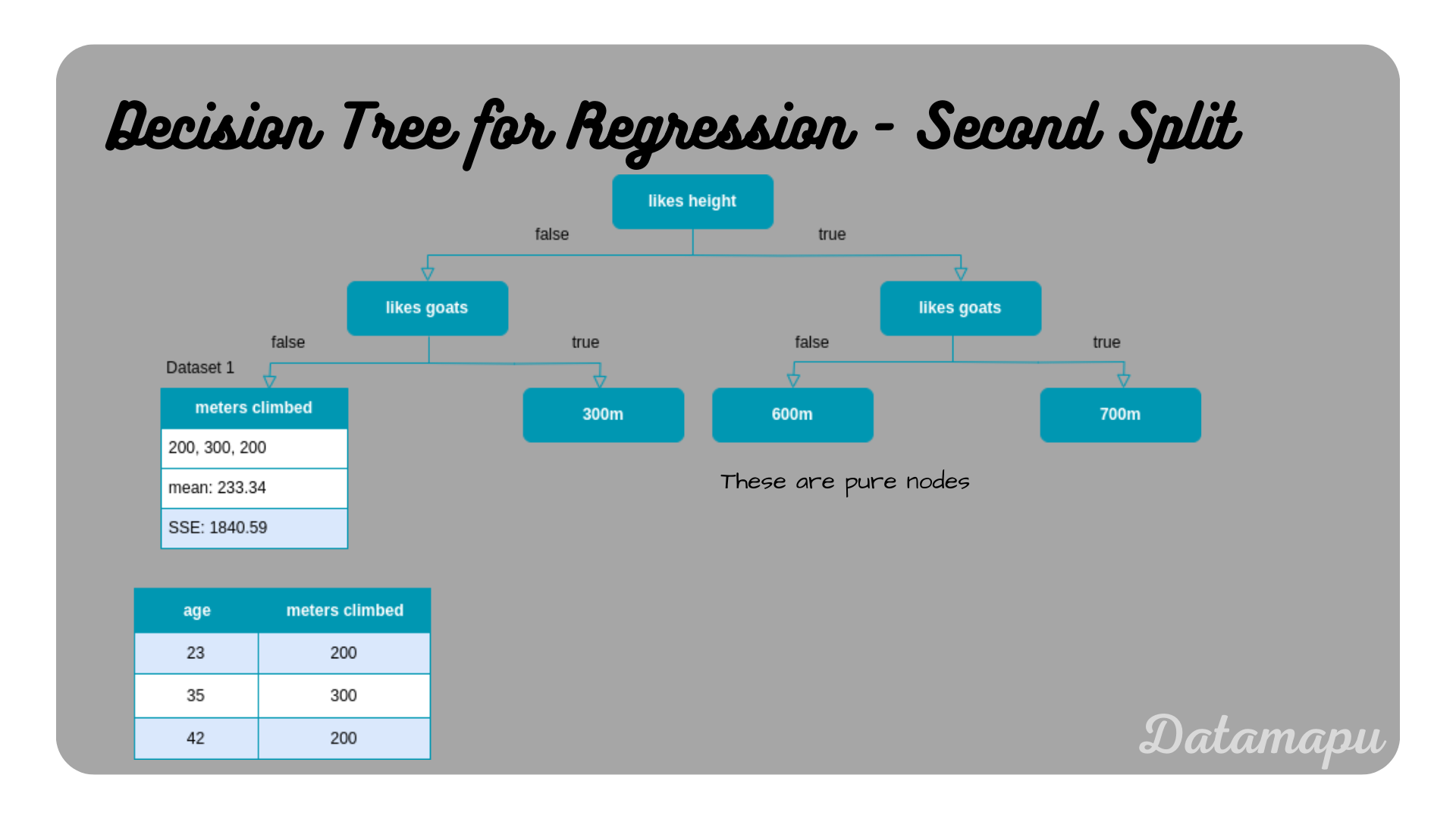The Decision Tree after the splits on the second level.

The resulting tree shows only one node that is not pure. Only the feature ‘age’ is left and two possible splits.

All possible splits for the third split.

Both possible splits result in the same SSE. That means we can use any of them. We will go on with ‘age = 29’. After that, only two items remain to split and we can build the final tree.

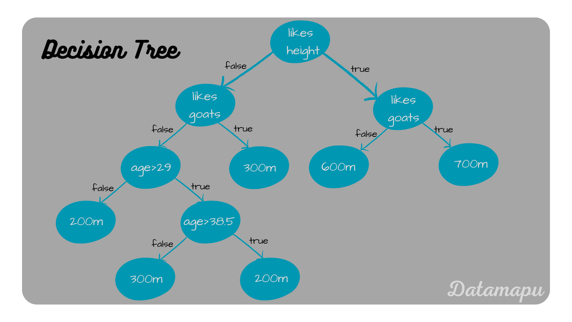Final Decision Tree.

Fit a Model in Python

In Python we can use the package sklearn to fit a Decision Tree model to our data.

 1
 2
 3
 4
 5
 6
 7
 8
 9
10
11
12
13
14
15
16

import pandas as pd
import matplotlib.pyplot as plt
from sklearn.tree import DecisionTreeRegressor

data = {'age': [23, 31, 35, 35, 42, 43, 45, 46, 46, 51], 
        'likes goats': [0, 1, 0, 0, 0, 1, 1, 1, 0, 1], 
        'likes height': [0, 1, 1, 0, 0, 1, 0, 1, 1, 1], 
        'climbed meters': [200, 700, 600, 300, 200, 700, 300, 700, 600, 700]}

df = pd.DataFrame(data)

X = df[['age', 'likes goats', 'likes height']].values
y = df[['climbed meters']].values.reshape(-1,)

reg = DecisionTreeRegressor()
reg = reg.fit(X, y)

We use the class DecisionTreeRegressor to fit a model and can visualize the fitted tree using sklearn.

1
2
3

from sklearn.tree import plot_tree

plot_tree(reg, feature_names=['age', 'likes goats', 'likes height'], fontsize=6)

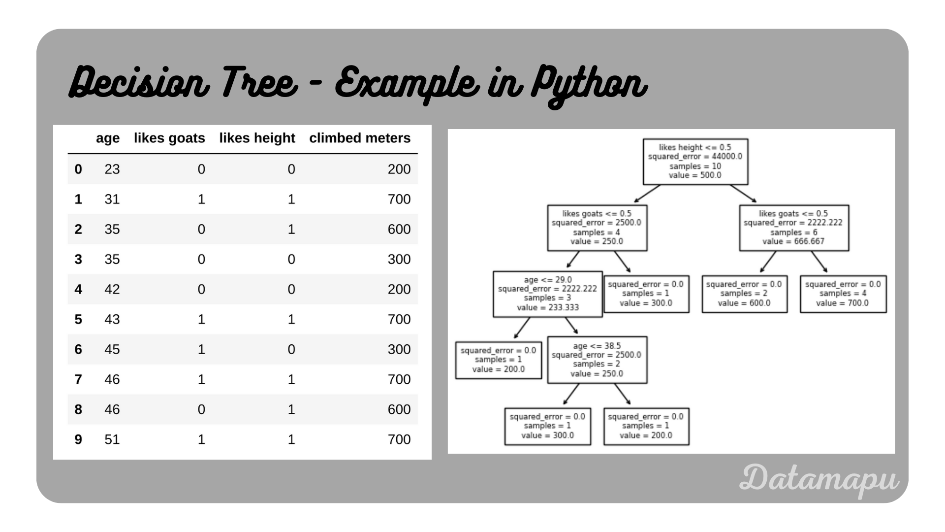Decision Tree build in Python.

Note, that there are some slight differences in the notation, but the resulting tree is the same as the one we developed above.

Summary

In this post, we developed a Decision Tree for a regression problem step by step. The most important step in building a Decision Tree is to find the best split. We used the SSE criterion, which is suitable for numerical data and is also the default method in sklearn. We then compared our results to the one we achieved using Python.

If this blog is useful for you, please consider supporting.

• Data Science
• Machine Learning
• Regression
• Decision Trees
• Tree Methods