Decision Trees - Explained
- 7 minutes read - 1463 wordsIntroduction
A Decision Tree is a supervised Machine Learning algorithm that can be used for both regression and classification problems. It is a non-parametric model, which means there is no specific mathematical function underlying to fit the data (in contrast to e.g. Linear Regression or Logistic Regression), but the algorithm only learns from the data itself. Decision Trees learn rules for decision making and used to be drawn manually before Machine Learning came up. They are hierarchical models, that have a flow-chart tree structure as the name suggests.
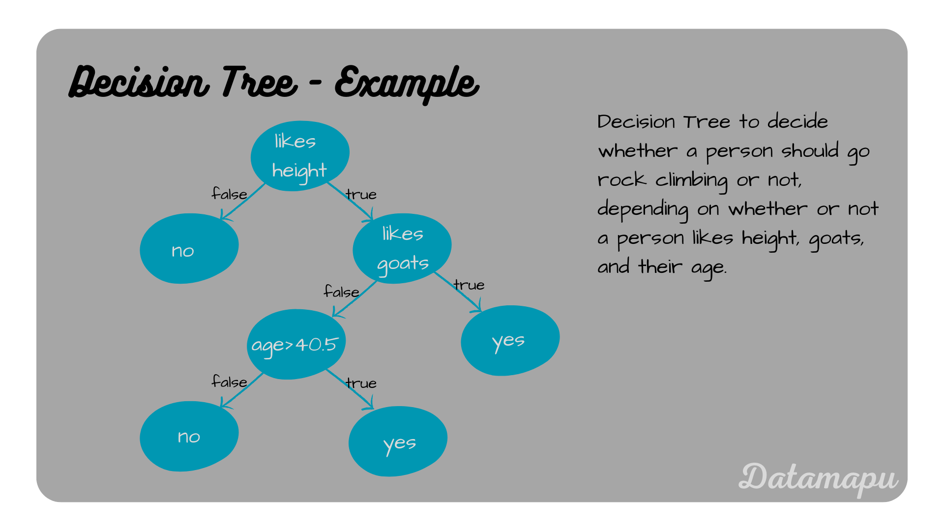
 Example for a Decision Tree.
Terminology
Before diving into the details of how to build a Decision Tree, let’s have a look at some important terms.
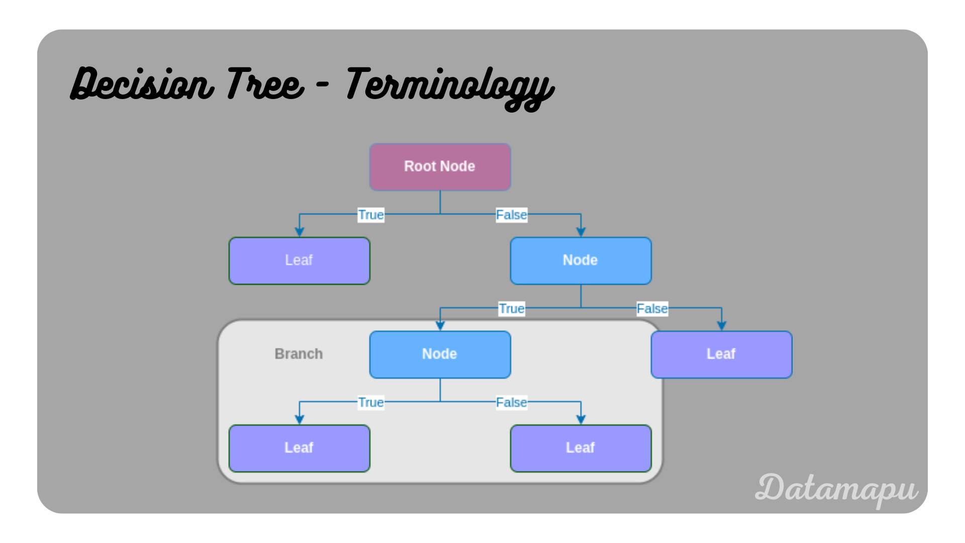
Root Node. The Root Node is the top-level node. It contains the entire dataset and represents the first decision.
Node. A node is also called an internal node or decision node. It represents a split into further (child) nodes or leaves.
Parent Node. A parent node is a node that precedes a (child) node.
Child Node. A child node is a node following another (parent) node.
Leaf. A leaf is also called a terminal node. It is a node at the end of a branch and has no following nodes. It represents a possible outcome of the tree, i.e. a class label or a numerical value.
Splitting. The process of dividing a node into two child nodes depending on a criterion and a selected feature.
Branches. A branch is a subset of a tree, starting at an (internal) node until the leaves.
Pruning. Removing a branch from a tree is called pruning. This is usually done to avoid overfitting.
 Illustration of the terminology of a Decision Tree.
Build a Tree
To develop a Decision Tree we start with the entire dataset and subsequently split it into smaller subsets. At each node, the dataset ($D$) is split into two subsets ($D_1$ and $D_2$) depending on the feature that best divides the labels by a specific criterion. Different splitting criteria exist, which depend on whether the labels are categorical (classification) or numerical (regression).
Splitting for Classification Tasks
Gini Impurity
The Gini Impurity for a split is calculated as
$$Gini(D) = \frac{n_1}{n} \cdot Gini(D_1) + \frac{n_2}{n} \cdot Gini(D_2),$$
with $n = n_1 + n_2$ the size of the dataset $D$, its subsets $D_1$, $D_2$, and
$$Gini(D_i) = 1 - \sum_{j=1}^c p_j^2,$$
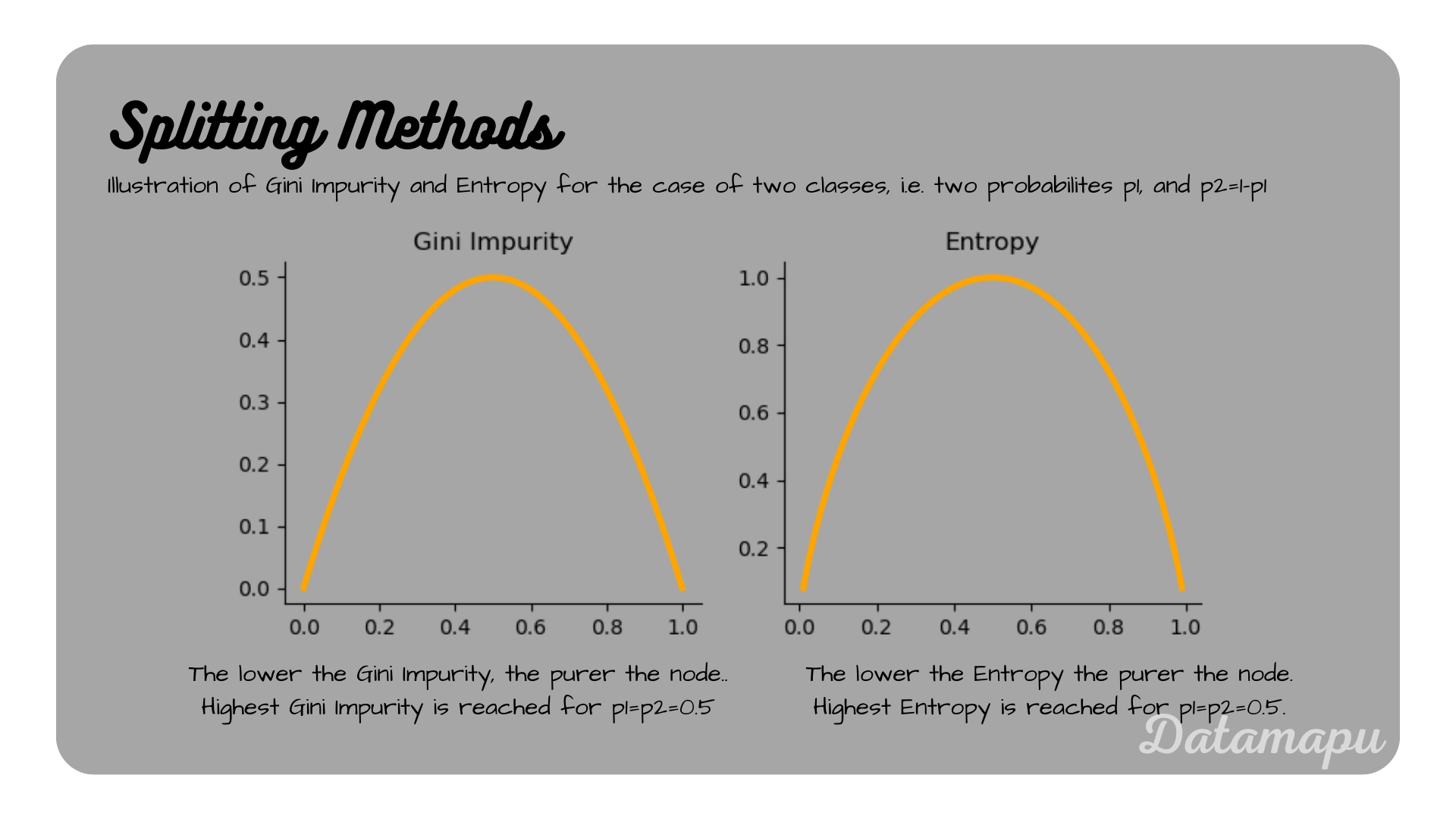
the Gini Impurity of node $i$. In this equation $p_j$ is the probability that a randomly drawn sample from this node belongs to class $j$ and $c$ the number of classes. The lower the Gini Impurity, the purer the node, or in other words the better the classes are separated. The Gini Impurity is calculated using the negative of the square of the probability, which by nature is a value between 0 and 1. That is, it is highest if the samples are uniformly distributed within a node. The Gini Impurity of a pure node is zero.
Follow these steps to split a Decision Tree based on Gini Impurity.
- For each possible split, create child nodes and calculate the Gini Impurity of each child node.
- Calculate the Gini Impurity of the split as the weighted average Gini Impurity of child nodes.
- Select the split with the lowest Gini Impurity.
Repeat steps 1–3 until no further split is possible. Note that possible splits may be more than features if the features are not all binary. A detailed example, where all the Gini Impurities of all splits are calculated and illustrated, can be found here.
Information Gain
The Information Gain is given by
$$Gain(D) = 1 - Entropy(D),$$
with
$$Entropy(D) = \frac{n_1}{n}\cdot Entropy(D_1) + \frac{n_2}{n}\cdot Entropy(D_2)$$
and
$$Entropy(D_i) = -\sum_{j=1}^c p_j log_2 p_j,$$
the Entropy of node $i$. In this equation $n = n_1 + n_2$ represent the sizes of the datasets $D$, $D_1$, and $D_2$. The lower the Entropy, the purer the node. Since the Entropy is subtracted from $1$, this means the higher the Information Gain, the purer the node.
Follow these steps to split a Decision Tree based on Information Gain.
- For each possible split, create child nodes and calculate the Entropy of each child node.
- Calculate the Entropy of the split as the weighted average Entropy of child nodes.
- Select the split with the lowest Entropy or highest Information Gain, respectively.
Repeat steps 1-3 until no further splits are possible.
Note, that a disadvantage of information Gain is, that it prefers features with a large number of classes, which may bias the splitting. A possibility to overcome this is to calculate the Information Gain Ratio instead. This is defined as
$$Gain Ratio = \frac{Gain}{-\sum_{j=1}^cp_jlog(p_j)}.$$
A detailed explanation is beyond the scope of this article. More information can be found here.
 Illustration of Gini Impurity and Entropy.
Splitting for Regression Tasks
Reduction in Variance
In this method the variance
$$\sigma^2_i = \frac{1}{n_i}\sum_{j=1}^{n_i}(x_j-\bar{x})^2$$
is used to determine the split. In the above formular $D_i$ represents the subset with size $n_i$. The lower the variance the purer the node. If a node only contains samples of the same value the variance is zero. That is in this case, we seek a low variance to find a good split.
Follow these steps to split a Decision Tree based on the reduction of variance.
- For each possible split, create child nodes and calculate the variance of each child node.
- Calculate the variance of the split as the weighted average variance of child nodes.
- Select the split with the lowest variance.
Repeat steps 1-3 until no further splits are possible.
Note, that an equivalent variant of calculating the reduction in variance is the calculation of the Sum of Squared Errors (SEE), which is defined as
$$SSE(D) = SSE(D_1) + SSE(D_2),$$
with
$$SSE(D_i) = \frac{1}{n_i}\sum_{j=1}^{n_i}(x_j-\bar{x}_i)^2.$$
Decision Trees in Python
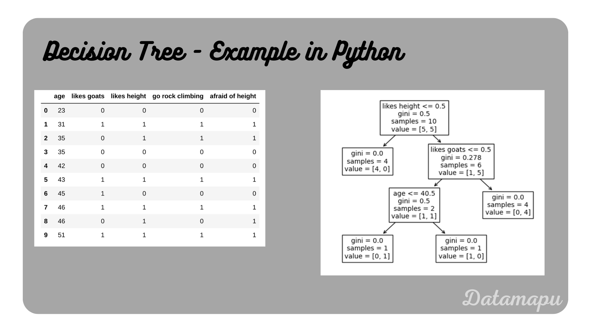
To determine a Decision Tree for a given dataset in Python, we can use the sklearn library. Both, Decision Trees for classification and regression tasks are supported. Here is a simple example for a classification problem. The splitting method used in sklearn is Gini Impurity. The task is to decide whether a person should go rock climbing or not, depending on whether the person likes height, goats, and their age, as illustrated at the beginning of this article.
| |
The class used to determine the Decision Tree is DecisionTreeClassifier. To get the predicted categories we can use the predict method. In this example, the result is y_hat = [0 1 1 0 0 1 0 1 0 1]. Accordingly, predict_proba gives the probability of each category. The Decision Tree can be illustrated in Python using the plot_tree class from sklearn.
| |
 Illustration of a Decision Tree in Python.
Advantages & Disadvantages
Advantages
- Decision Trees are intuitive, easy to implement, and interpret.
- Decision Trees are not affected by outliers, missing values, or co-linearity between features.
- Decision Trees can be used with numerical and categorical data
- The data doesn’t need to be scaled.
- As non-parametric algorithms, Decision Trees are very flexible.
Disadvantages
- Decision Trees tend to overfit. To overcome this, pruning the tree may help.
- Decision Trees cannot predict continuous variables. That is also when applied to a regression problem the predictions must be separated into categories.
- As a non-parametric algorithm, the training of a Decision Tree may be expensive if the dataset is large.
Summary
In this article, we learned what Decision Trees are and how to build them depending on whether a regression or a classification problem is considered. We considered a selection of splitting criteria, there are of course many more. Decision Trees are powerful Machine Learning models with some major advantages such as easy interpretability and robustness against missing values. A main disadvantage of Decision Trees is that they easily overfit and have difficulties in generalizing to unseen data. In the article Decision Tree Example for Classification, you can find a detailed calculation by hand of the above developed Decision Tree. For a more realistic example with a larger dataset, you can find a notebook on kaggle. In a separate article, you can find the development of a Decision Tree Example for Regression.
If this blog is useful for you, please consider supporting.
