Linear Regression - Explained
- 7 minutes read - 1470 wordsIntroduction
Linear Regression is a type of Supervised Machine Learning Algorithm, where a linear relationship between the input feature(s) and the target value is assumed. Linear Regression is a specific type of regression model, where the mapping learned by the model describes a linear function. As in all regression tasks, the target variable is continuous. In a linear regression, the linear relationship between one (Simple Linear Regression) or more (Multiple Linear Regression) independent variable and one dependent variable is modeled.
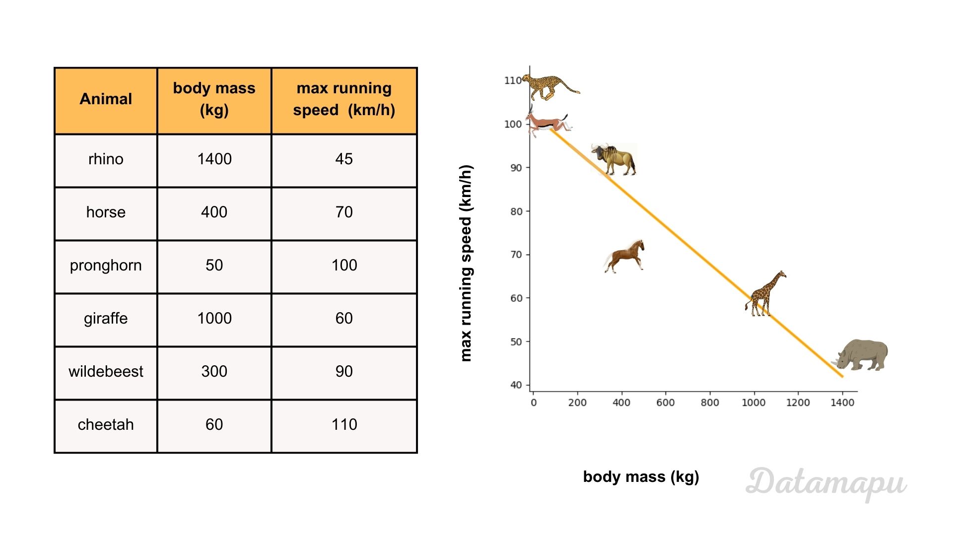 Illustration of a simple linear regression between the body mass and the maximal running speed of an animal.
Simple Linear Regression
A Simple Linear Regression describes a relationship between one independent variable (input feature, $x$) and one dependent variable (target value, $y$). This relationship is modeled by a linear equation. The objective is to find the linear line that fits the data best, in the sense of minimizing the error between the predicted values and the actual values. A linear regression model follows the equation $$\hat{y} = a\cdot x + b.$$ In this equation $\hat{y}$ is the predicted estimate of $y$, $a$ the slope, which represents the change of the dependent variable ($y$) depending on the independent variable ($x$) and $b$ is the intercept, that gives the value of the dependent variable ($y$) for the case the independent variable is zero ($x=0$). The most important terms are illustrated in the following plot.
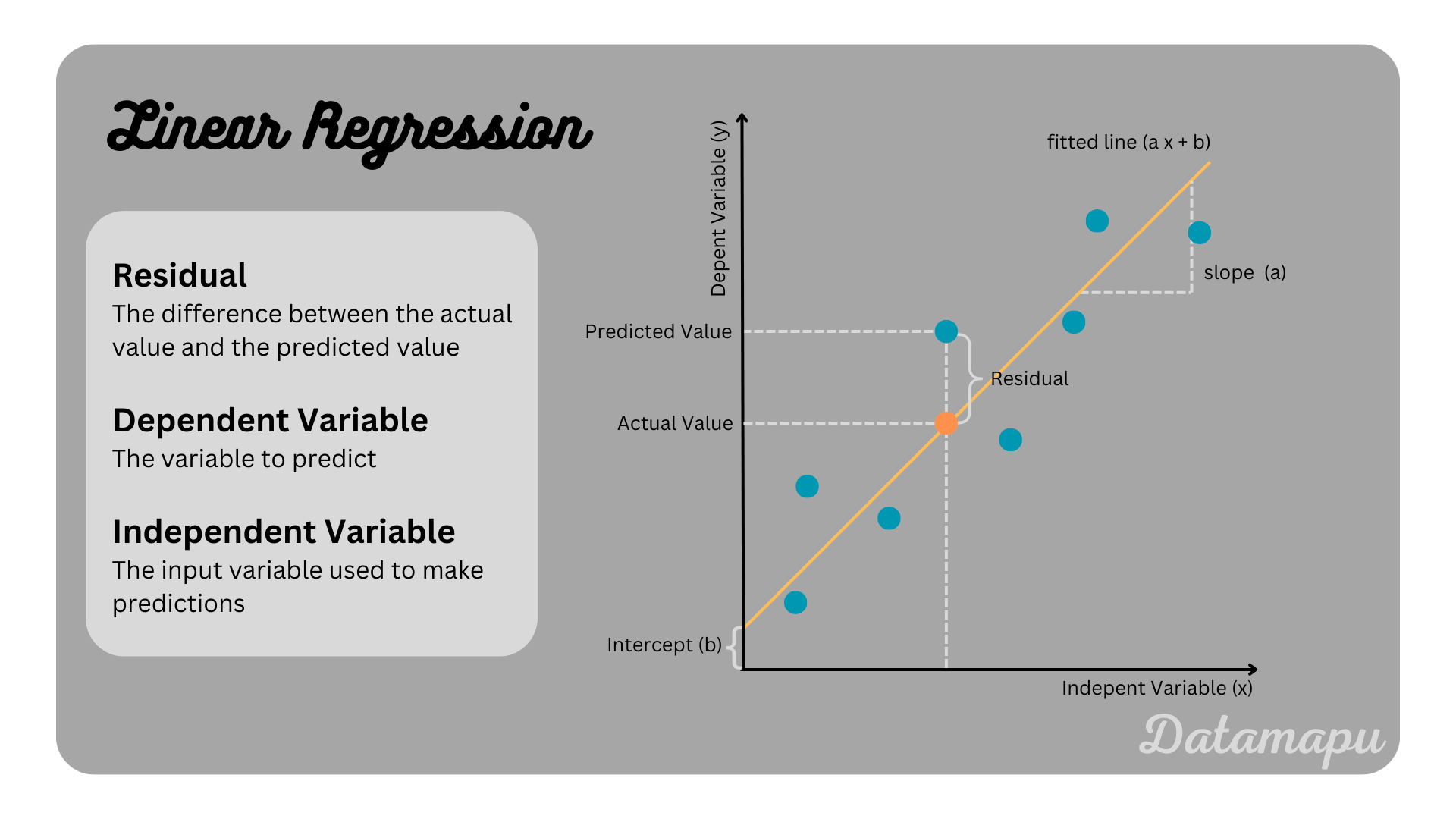 Illustration of a simple linear regression.
Find the best Fit
As in every Machine Learning algorithm, in order to find the best fit the error between the actual values and the predicted values is minimized. This error is described by a loss function. In a linear regression, the loss function is usually the Mean Squared Error
$$MSE = \frac{1}{N}\sum_{i=1}^{N}(y_i-\hat{y_i})^2,$$
with $y$ representing the actual value and $\hat{y}$ the prediction. When plugging in the equation for the linear model we get $$MSE = L(a, b) = \frac{1}{N}\sum_{i=1}^{N}(y_i - (a\cdot x_i +b))^2.$$
To find a linear model we need to determine the slope $a$ and the intercept $b$, such that the loss function (here the MSE) is minimized. One popular minimization technique is the Gradient Descent. The Gradient Descent is a process, in which the parameters $a$ and $b$ are iteratively updated. Starting with random values the values $a$ and $b$ are updated in each step to achieve an optimized solution. To reach a minimum with this strategy, the parameters have to be updated in the correct direction. The gradient of a function describes the direction of the steepest ascent, that is in order to find the minimum we need to update the parameters in the direction of the negative of the gradient. The gradient is determined by the partial derivatives with respect to $a$ and $b$
$$\frac{\delta{L}}{\delta a}= \frac{2}{N} \sum_{i=1}^N (y_i -a \cdot x_i - b)\cdot (-x_i)$$ $$\frac{\delta{L}}{\delta b}= \frac{2}{N} \sum_{i=1}^N (y_i -a \cdot x_i - b)\cdot (-1).$$
The stepsize of the update is defined by the learning rate $\alpha$. The updating rule, then takes the form
$$w_{i+1} = w_{i} + \alpha \nabla L.$$
If $\alpha$ is chosen very large the minimum may be missed, if it is very small finding the minimum and with that the training may take long, as illustrated in the next plot.
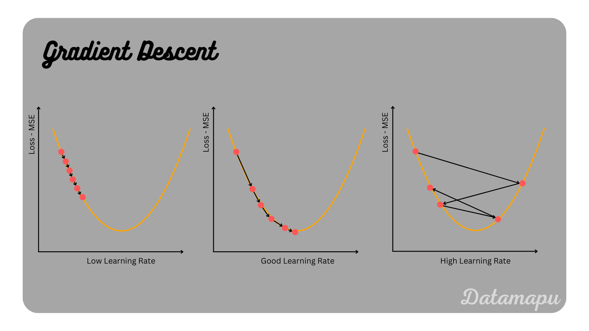 Illustration of gradient Descent for different learning rates.
Note, that for a linear regression, the minimum can also be calculated analytically by setting the derivatives to zero and deriving the coefficients from these equations. This is however computationally more expensive, especially when multiple independent variables (Multiple Linear Regression) are considered.
Multiple Linear Regression
In multiple linear regression a linear relationship two or more independent variables (input features, $x_1$, $x_2$, $\dots$, $x_n$) and one dependent variable (target value, $y$) is described $$\hat{y} = a_0 + a_1\cdot x_1 + a_2\cdot x_2 + \dots + a_n \cdot x_n.$$ As previously, $\hat{y}$ estimates the dependent variable $y$. In a Multiple Linear Regression the independent variables can be either numerical or categorical.
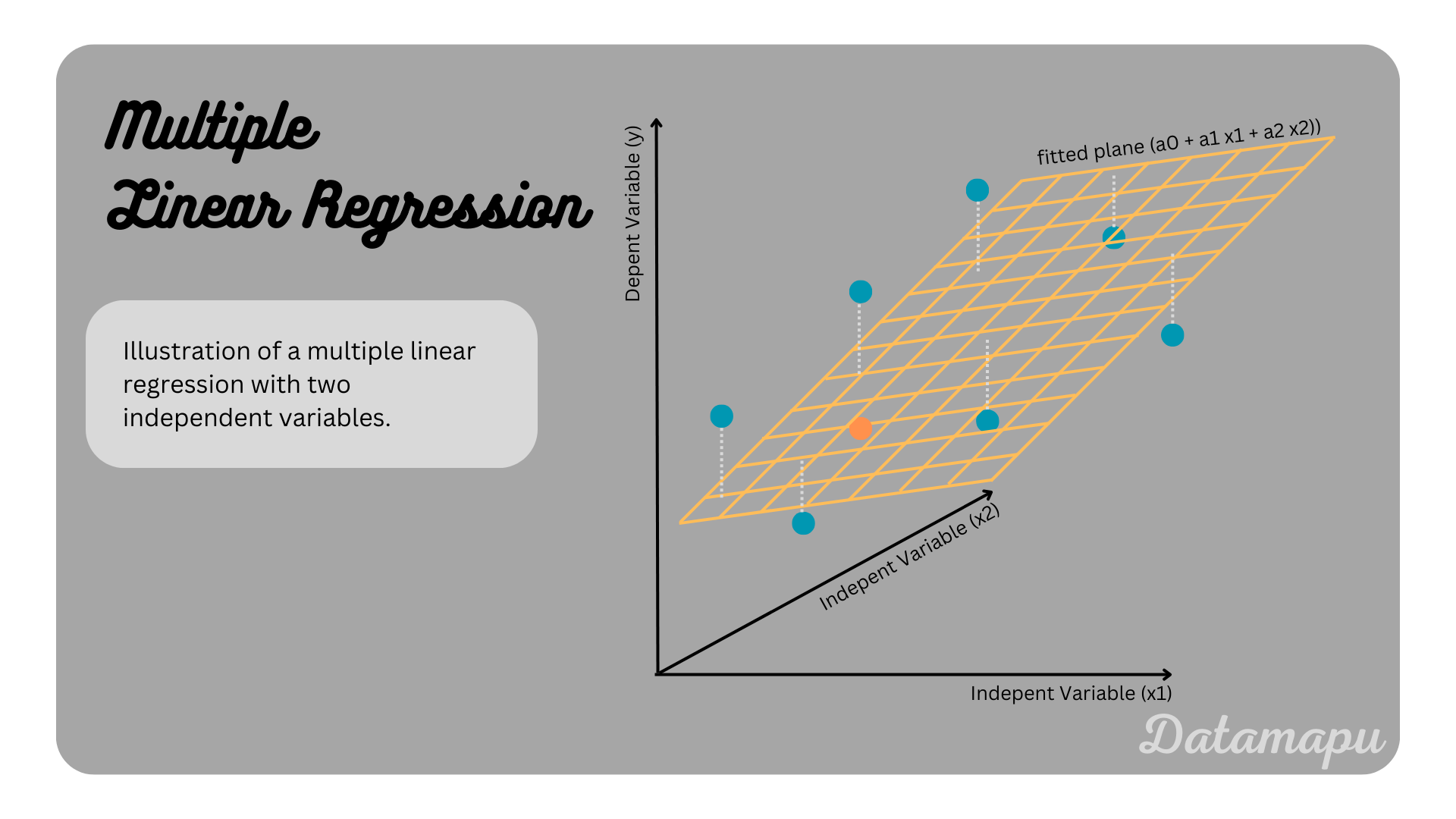 Illustration of a multiple linear regression with two indepent variables.
Asumptions
To reasonable perform a linear regression the data need to fulfill the following criteria:
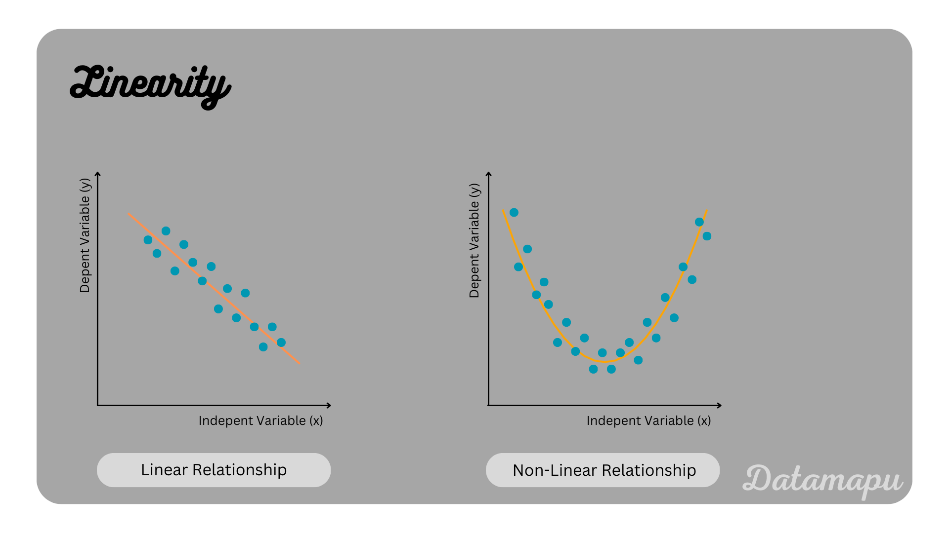
Linearity. The dependent variable ($x$) and the independent variability ($y$) should have a linear relationship. To determine if that is true the data can be visualized in a scatterplot. This can also be used to identify outliers, which should be removed. A linear regression is sensitive to outliers and they may adulterate the results.
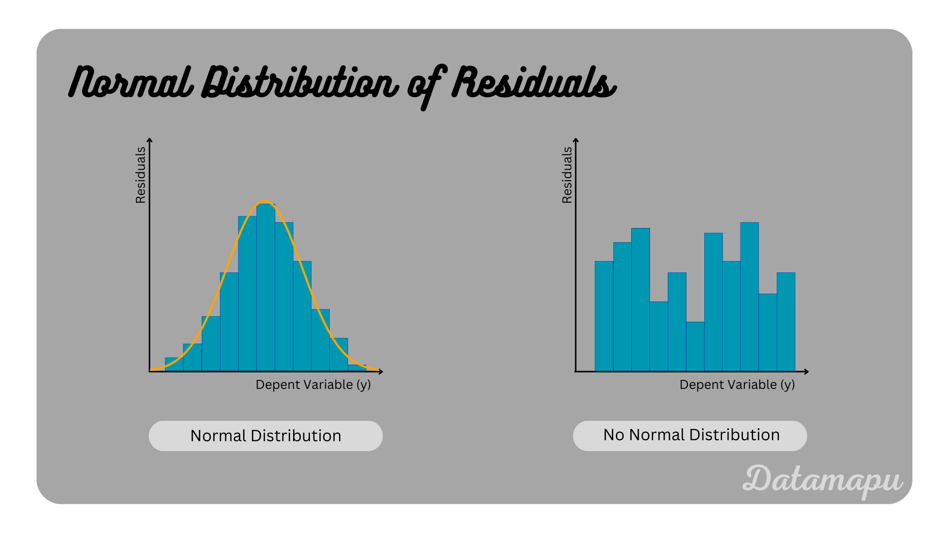
Normal Distribution of Residuals. The distribution of the residuals should be normally distributed. This assures that the model captures the main pattern of the data.
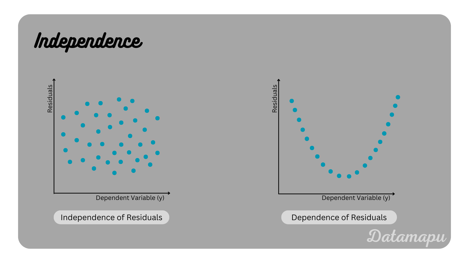
Independence. The independent variables are not dependent of each other. In other words, there is no autocorrelation within the dependent data.
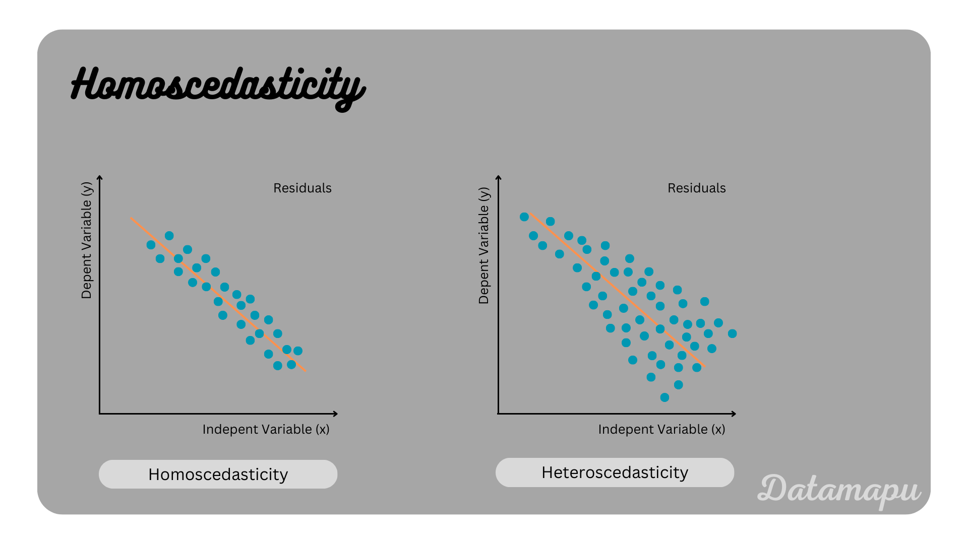
Homoscedasticity. The variance of the residuals is constant. This especially means that the number of datapoints has no impact on the variance of the residuals.
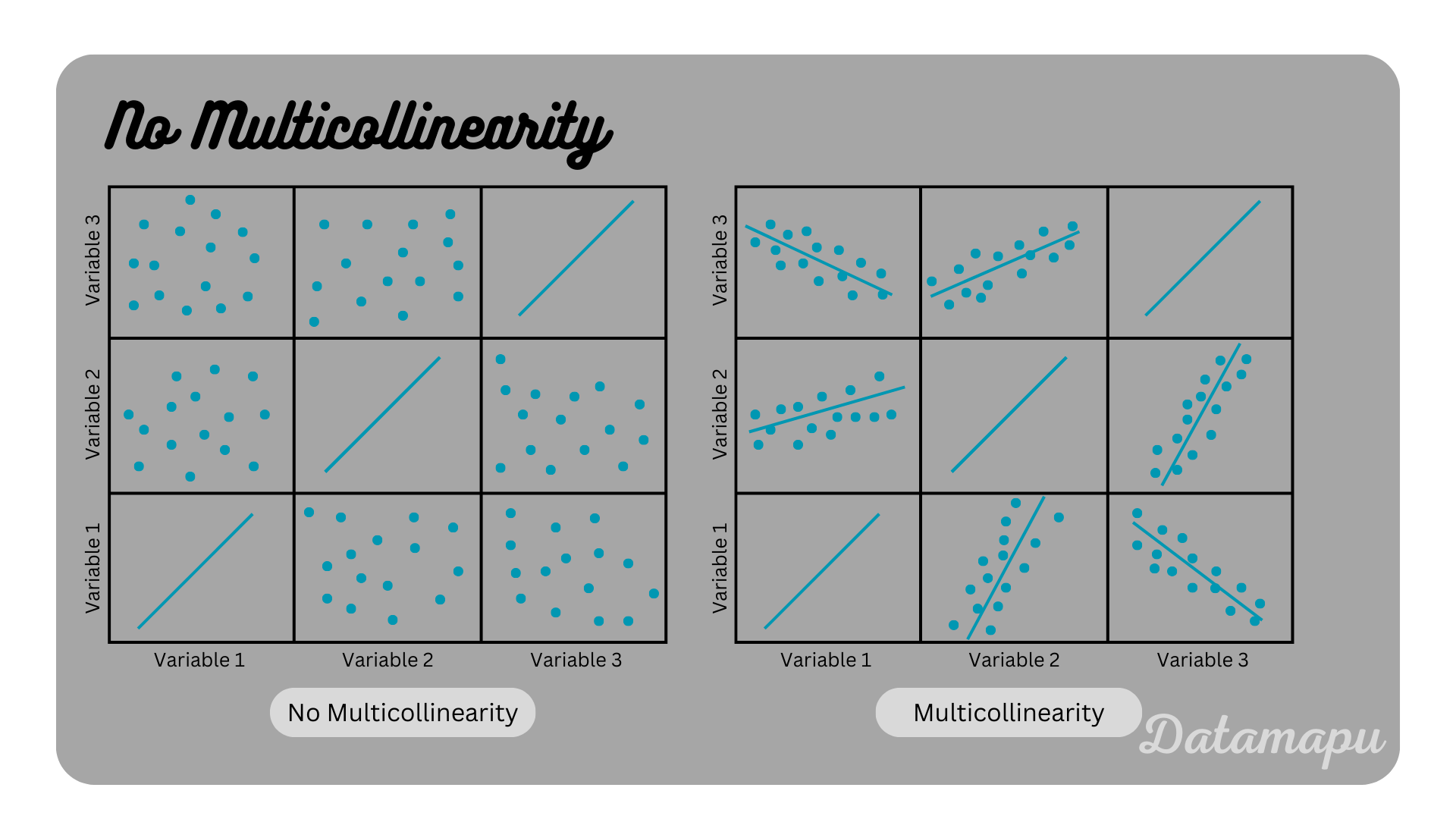
No Multicollinearity. If more than one independent variable is used, the correlation between the different independ variables should be low. Highly correlated variables make it more difficult to determine the contribution of each variable individually.
Evaluation
After fitting a model, we need to evaluate it. To evaluate a linear regression the same metrics as for all regression problems can be used. Two very common ones are Root Mean Squared Error (RMSE) and Mean Absolute Error (MAE). Both metrics are based on the difference between the predicted and the actual values, the so-called Residuals. The MAE is defined as the sum of the absolute values of the residuals for all data points, divided by the total number of data points. The RMSE is defined as the square root of the sum of the squared residuals divided by the total number of data points. Both metrics avoid the elimination of errors by taking the absolute value and the square accordingly and are easy to interpret because they carry the same units as the target variable. The RMSE, due to taking the square, helps to reduce large errors. A more detailed overview and description of these and other common metrics for regression is given in a separate article.
Advantages
The main advantage of a Linear Regression is its interpretability. The coefficients - in a simple Linear Regression the slope - describe the influence of the (numerical) input (independent) variable to the target (dependent) variable. That is the coefficients can be interpreted as the strength this specific input variable has on the target variable. Confidence intervals of the coefficients can be calculated to estimate their reliability. If in a multiple linear regression a categorical feature is included, the target variable increases if this variable is a specific category.
Another advantage is easy implementation. The Linear Regression is the simplest Machine Learning model for a regression problem, which can be implemented much easier than other - more complex models - and is therefore also scalable.
Disadvantages
Linear Regression is sensible to outliers. That is outliers can impact a Linear Regression Model significantly and lead to misleading results. In real life relationships between variables are rarely linear, which means a Linear Regression tends to oversimplify this relationship.
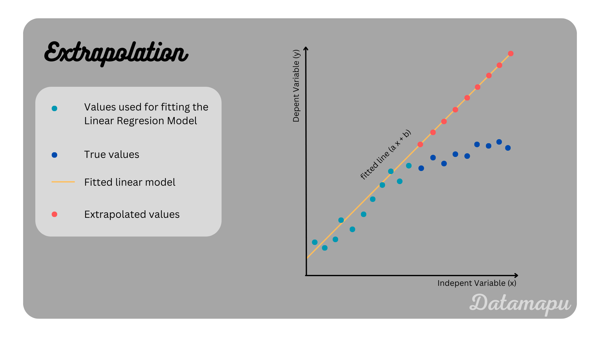
Extrapolation of a Linear Regression should be done with a lot of caution. The prediction of values outside of the values the model was trained on is often inappropriate, and may yield misleading predicions, as illustrated in the following plot.
Linear Regression in Python
When implementing a Linear Regression in Python, we can use the sklearn library, as demonstrated in the following simplified code example. The relationship described is $y = 2\cdot x +3$, with some noise added to $y$.
| |
This yields to $a = 1.93$ for the slope, and $b = 3.23$ for the intercept. The predictions are given by $\hat{y} = [5.16, 7.09, 9.02, 10.95, 12.88]$.
Summary
Linear Regression is a simple, yet powerful tool in supervised Machine Learning. Its power is mainly its simplicity and interpretability. These two reasons make it popular in academic and business use cases. However, it is important to know its limitations. In real life most relationships are not linear and applying a Linear Regression to such data, may lead to misleading and wrong results.
You can find a simplified example for a Simple Linear Regression where the analytical solution for the slope and the intercept is developed by hand in the separate article Linear Regression - Analytical Solution and Simplified Example. A more realistic tutorial for a linear regression model, predicting house prices in Boston using a Simple and a Multiple Linear Regression is elaborated in a notebook on kaggle
If this blog is useful for you, please consider supporting.
