Linear Regression - Analytical Solution and Simplified Example
- 5 minutes read - 883 wordsIntroduction
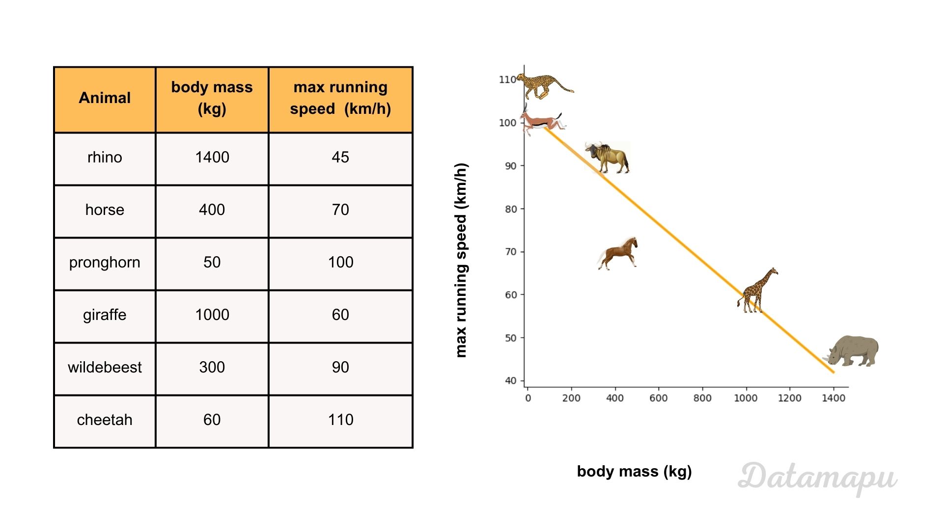
In a previous article, we introduced Linear Regression in detail and more generally, showed how to find the best model and discussed its chances and limitations. In this post, we are looking at a concrete example. We are going to calculate the slope and the intercept from a Simple Linear Regression analytically, looking at the example data provided in the next plot.
 Illustration of a simple linear regression between the body mass and the maximal running speed of an animal.
Fit the Model
We aim to fit a model that describes the relationship between the body mass (independent variable / input feature $x$) and the speed (dependent / target variable $y$) of the animals, following the equation
$$\hat{y} = a\cdot x + b,$$
with $\hat{y}$ approximating the target values $y$. In order to find this model, we need to determine the coefficients $a$ and $b$. As we learned in the article about Linear Regression, In order to fit a Linear Regression model, we need to minimize the error between the predictions and the actual values. In Machine Learning this error, depending on the parameters of the model is often called the Loss-Function. For a Simple Linear Regression, these parameters are the slope ($a$) and the intercept ($b$). Usually, the Mean Squared Error is used as Loss-Function in Linear Regression
$$MSE = L(a, b) = \frac{1}{N}\sum_{i=1}^{N}(y_i - (a\cdot x_i +b))^2.$$
Minimize the Loss
In real applications optimization techniques, such as Gradient Descent are used to estimate the minimum of the Loss Function. In this article, we will calculate the coefficients $a$ and $b$ analytically. As we know from calculus a criterion required for a minimum is that the gradient is zero. The gradient is compiled by the partial derivatives. Following the chain rule, the partial derivatives of $L$ with respect to $a$ and $b$ are
$$\frac{\delta{L}}{\delta a}= \frac{2}{N} \sum_{i=1}^N (y_i -a \cdot x_i - b)\cdot (-x_i)$$ $$\frac{\delta{L}}{\delta b}= \frac{2}{N} \sum_{i=1}^N (y_i -a \cdot x_i - b)\cdot (-1).$$
Setting these equations to zero and multiplying both sides with $-1$, we get
$$0 = \frac{2}{N} \sum_{i=1}^N (y_i -a \cdot x_i - b)\cdot x_i$$ $$0 = \frac{2}{N} \sum_{i=1}^N (y_i -a \cdot x_i - b)$$
We will start with the second equation and resolve it for $b$
$$\sum_{i=1}^N b = \sum_{i=1}^N y_i - a\cdot \sum_{i=1}^N x_i$$
$$N \cdot b = \sum_{i=1}^N y_i - a \sum_{i=1}^N x_i$$
$$b = \frac{1}{N} \sum_{i=1}^N y_i - a \frac{1}{N} \sum_{i=1}^N x_i$$
$$b = \bar{y} - a\cdot \bar{x},$$
with $\bar{x} = \sum_{i=1}^N x_i$ and $\bar{y} = \sum_{i=1}^N y_i$.
Now, we continue with the first equation and resolve it for $a$
$$0 = \sum_{i=1}^N(y_i - a\cdot x_i -b)x_i.$$
We use the equation we resolved for $b$ and plug it into this equation, which leads to
$$0 = \sum_{i=1}^N (y_i - a \cdot x_i - b)\cdot x_i$$
$$0 = \sum_{i=1}^N (y_i - a \cdot x_i -(\bar{y} - a\cdot\bar{x}))\cdot x_i$$
$$0 = \sum_{i=1}^N (y_i - \bar{y} - a\cdot(x_i - \bar{x}))\cdot x_i$$
$$0 = \sum_{i=1}^N x_i (y_i - \bar{y}) - \sum_{i=1}^N a\cdot x_i\cdot(x_i - \bar{x})$$
$$\sum_{i=1}^N x_i \cdot (y_i - \bar{y}) = a\cdot \sum_{i=1}^N x_i\cdot(x_i - \bar{x})$$
$$a = \frac{\sum_{i=1}^N x_i\cdot(y_i - \bar{y})}{\sum_{i=1}^Nx_i\cdot(x_i - \bar{x})}.$$
With that, we can calculate the coefficients $a$ and $b$ that determine the Simple Linear Regression model, we aim to develop.
Note, as we know from calculus setting the first derivative, i.e. the gradient to zero is not a sufficient condition for a minimum. For this example, we assume that the only location with zero gradient is a minimum. To be sure that this is really a minimum we would need to check all second derivatives. At this point, it could also be a maximum or a saddle point. This is however not the scope of this article.
Example
We now use the data presented above to determine the linear relationship between the size and the speed of an animal, represented by
$$\hat{y} = a \cdot x + b,$$
with $\hat{y}$ estimating the maximal running speed ($y$) and $x$ being the body mass. We start with calculating the means $\bar{x}$ and $\bar{y}$, with
$$x = [1400, 400, 50, 1000, 300, 60]$$ $$y = [45, 70, 100, 60, 90, 110].$$
This results in
$$\bar{x} = \frac{1400 + 400 + 50 + 1000 + 300 + 60}{6} = \frac{3210}{6} = 535$$ $$\bar{y} = \frac{45 + 70 + 100 + 60 + 90 + 110}{6} = \frac{475}{6} = 79.17.$$
With that we can calculate
$${\small a = \frac{1400\cdot (45 - 79.17) + 400\cdot (70 - 79.17) + 50\cdot (100 - 79.17) + 1000\cdot (60 - 79.17) + 300\cdot (90 - 79.17) + 60\cdot (110 - 79.17)}{1400\cdot (1400 - 535) + 400\cdot (400 - 535) + 50\cdot (50 - 535) + 1000\cdot (1000 - 535) + 300\cdot (300 - 535) + 60\cdot(60 - 535)}},$$
which gives
$$a = -0.043,$$
rounded up to 3 digits. With this we can calculate
$$b = \bar{y} - a\cdot\bar{x} = 79.17 + 0.043\cdot 535 = 102.175.$$
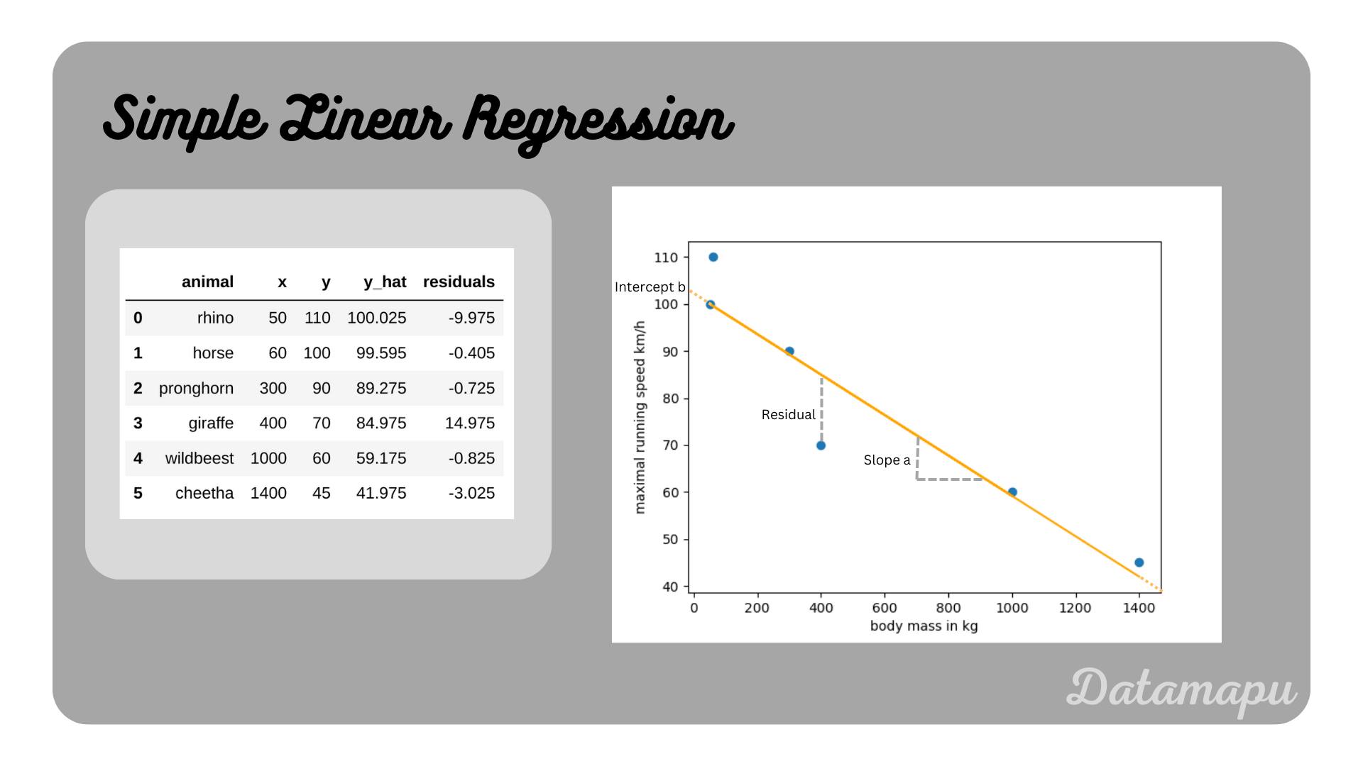
The resulting linear regression model and the original data is illustrated in the following plot.

Note, for this simplified example, we are not going to check the assumptions that need to be fulfilled for a Linear Regression. This example is only for illustration purposes, with this little amount of data statistical tests are not reasonable.
If this blog is useful for you, please consider supporting.
