Introduction to Deep Learning

November 2, 2023 - 11 minutes read - 2248 words

In this article we will learn what Deep Learning is and understand the difference to AI and Machine Learning. Often these three terms are used interchangeable. They are however not the same. The following diagram illustrates how they are related.

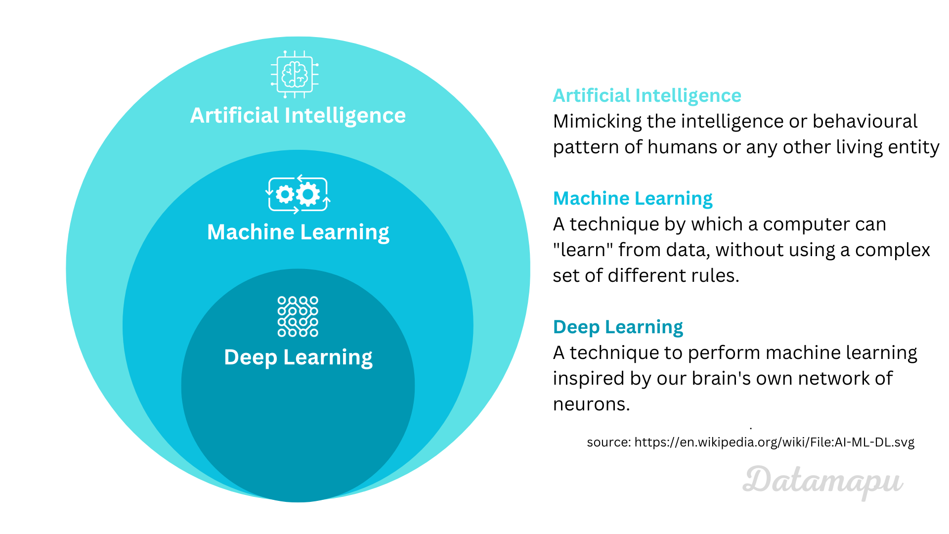ai_ml_dl Relation of Artificial Intelligence, Machine Learning and Deep Learning.

Artificial Intelligence. There are different definitions of Artificial Intelligence, but in general, they involve computers performing tasks that are usually associated with humans or other intelligent living systems. This is the definition given on Wikimedia: It says: “[AI is] Mimicking the intelligence or behavioral pattern of humans or any living entity”

Machine Learning. Machine learning is a subset of Artificial Intelligence. It describes the process where a computer can “learn” from data, without a given set of rules. In practice, these terms are often not well distinguished. People often talk about ML, but refer to it as AI.

Deep Learning. Deep Learning is a particular type of Machine Learning, which uses Neural Nets as models. Neural Nets were inspired by the way neurons in our brain work.

Classical Programming vs. Machine Learning

In this article we are going to learn about Deep Learning, which, as we just saw, is a subset of Machine Learning. Machine Learning differs conceptionally from classical programming. In classical programming we use data and rules to get the answers to a problem. In contrast, in Machine Learning we use the data and the answers to a problem to achieve the rules. This is illustrated in the following chart.

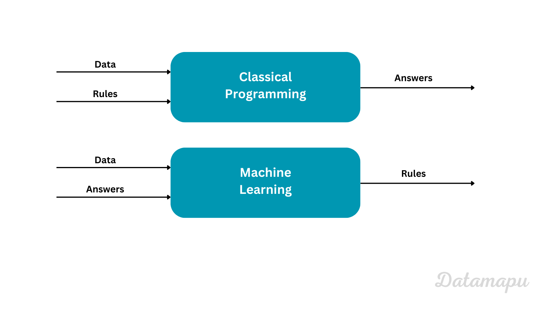ai_ml_dl Classical programming vs. Machine Learning.

What is a Neural Net?

A Neural Net is a special type of Machine Learning model which is used for Deep Learning. It is often illustrated as shown in the next plot. The name and structure of a Neural Net are inspired by the human brain, mimicking the way that biological neurons signal to one another. However, other than inspiration and naming, they are actually not very similar. A neural network consists of connected computational units, which are called neurons.

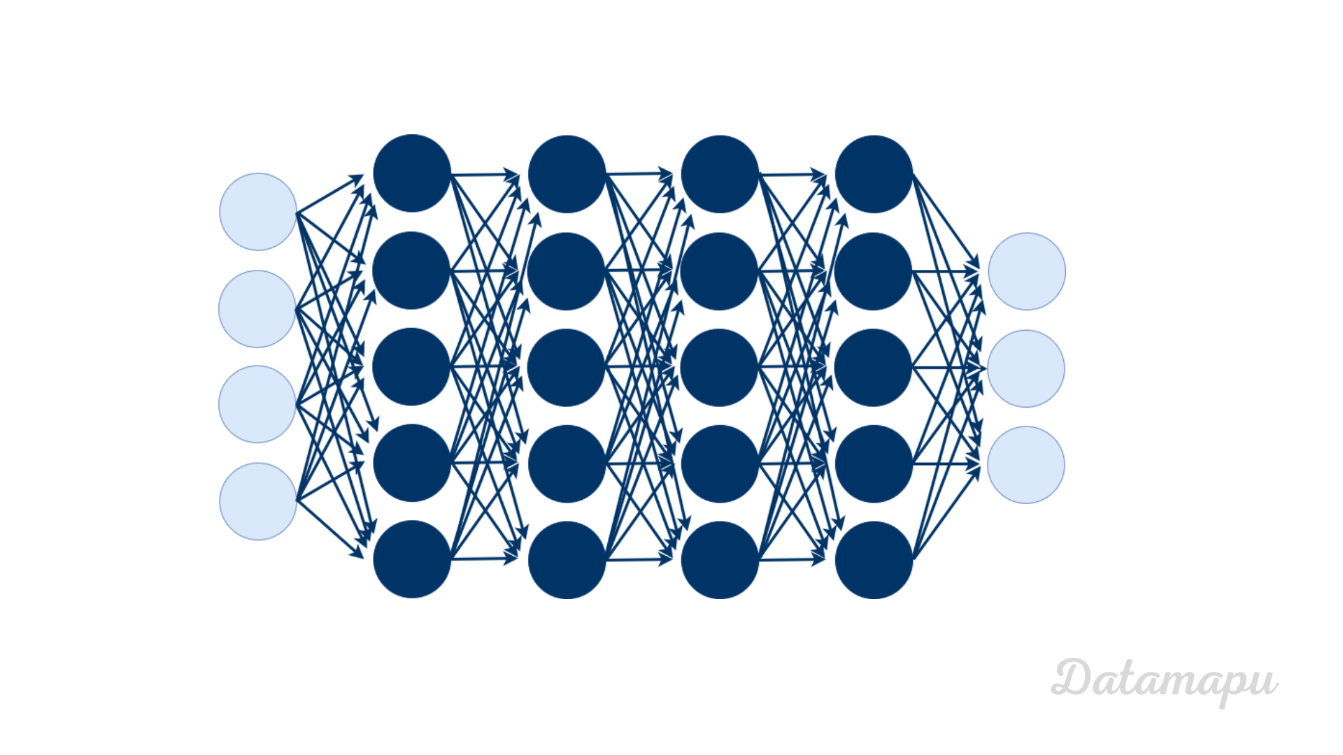ai_ml_dl Illustration of a Neural Net.

Neuron

Let’s zoom in and understand how a neuron works. The following plot illustrates a single neuron in more detail. Each neuron has one or more floating point inputs, the so-called input data, here shown as $x_1$ to $x_n$. Each of these input numbers is multiplied by a weight - $w_1$ to $w_n$. Then the weighted sum of the inputs is taken and additionally, an extra constant weight, which is the bias term, is added, here shown as $b$. These weights ($w_1$ to $w_n$) are learned during the training of the Neural Net. We will discuss how this exactly works later. Next, a non-linear function - the so-called activation function, is applied to this sum. This is a pre-defined function and we will see in the next paragraph what such an activation function looks like. Finally, the neuron returns an output value, which is also a floating point number.

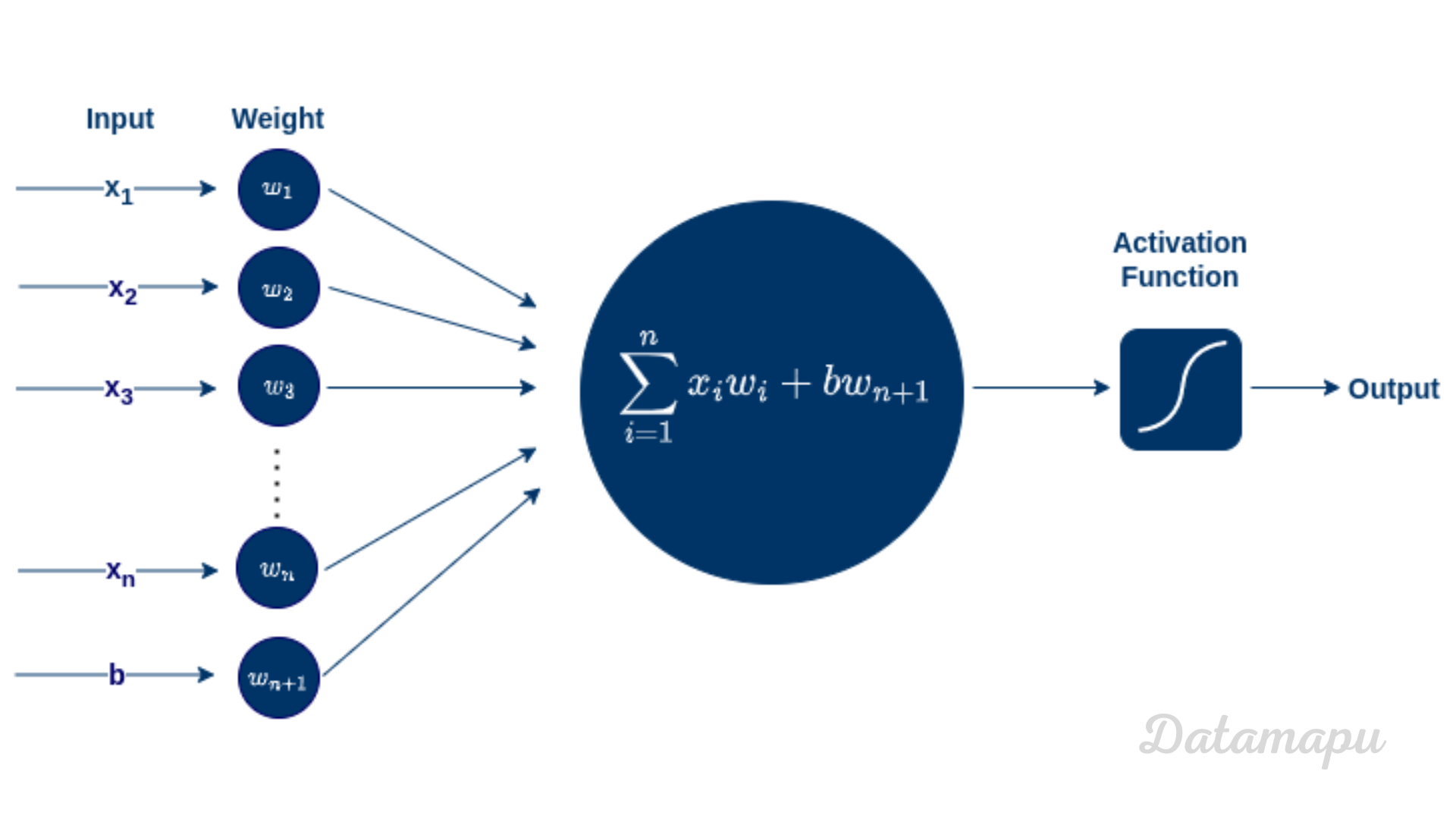ai_ml_dl Illustration of one Neuron of a Neural Net.

Activation Function

The purpose of the activation function is to introduce non-linearity into the output of a neuron. A Neural Network without an activation function is essentially just a linear regression model. The activation function does the non-linear transformation to the input, making it capable to learn and perform more complex tasks. Some typical activation functions are:

The Binary Stepfunction is $0$ for $x <= 0$ and $1$ elsewhere. This is one of the simplest activation functions. A threshold value is used to decide whether a neuron is activated or not. If the input is greater than a certain threshold, the neuron is activated, else it is not activated. If it is not activated, the output is not passed on to the next hidden layer. The binary stepfunction can only be used for binary classification and not for multiple classification problems. Further, the gradient of this activation function is $0$, which means it should not be used in a hidden layer, but only in the output layer.

The Rectified Linear Unit, or short ReLU, is $0$ for $x <= 0$ and $x$ elsewhere this is one of the most commonly used activation functions. With the ReLU function, only neurons are activated when the input of the activation function is positive. That is, not all neurons are activated at the same time. This fact makes the ReLU computationally efficient. However, it may also result in so-called “dead neurons” - i.e. neurons that are never activated.

The Leaky ReLU is similar to the ReLU but it has a small slope for negative values. This activation function is preferred when we may have sparse gradients. The Leaky ReLU overcomes the problems of the ReLU activation function, that some neurons are never activated.

The output of the Sigmoid activation function is between $0$ and $1$. It is preferred when the output is a probability. The Sigmoid-activation function is differentiable with a smooth gradient. A disadvantage is that the gradient tends to vanish, because the derivative of the sigmoid function is flat. Also, the sigmoid function is not symmetric around $0$, which makes the training of a Neural Net more complicated. It is preferred to be used for the output layer and not for hidden layers.

Similar, but going from $-1$ to $1$ is the Hyperbolic Tangent (Tanh). Compared to the sigmoid function, the Tanh is centered around $0$. It is usually used in hidden layers, as it helps to center the data. It has the same issue considering vanishing gradients as the sigmoid activation function.

Also similar is the Inverse Tangent function (ArcTan), which goes from $-π/2$ to $π/2$. It has the same advantages and disadvantages as the Tanh activation function.

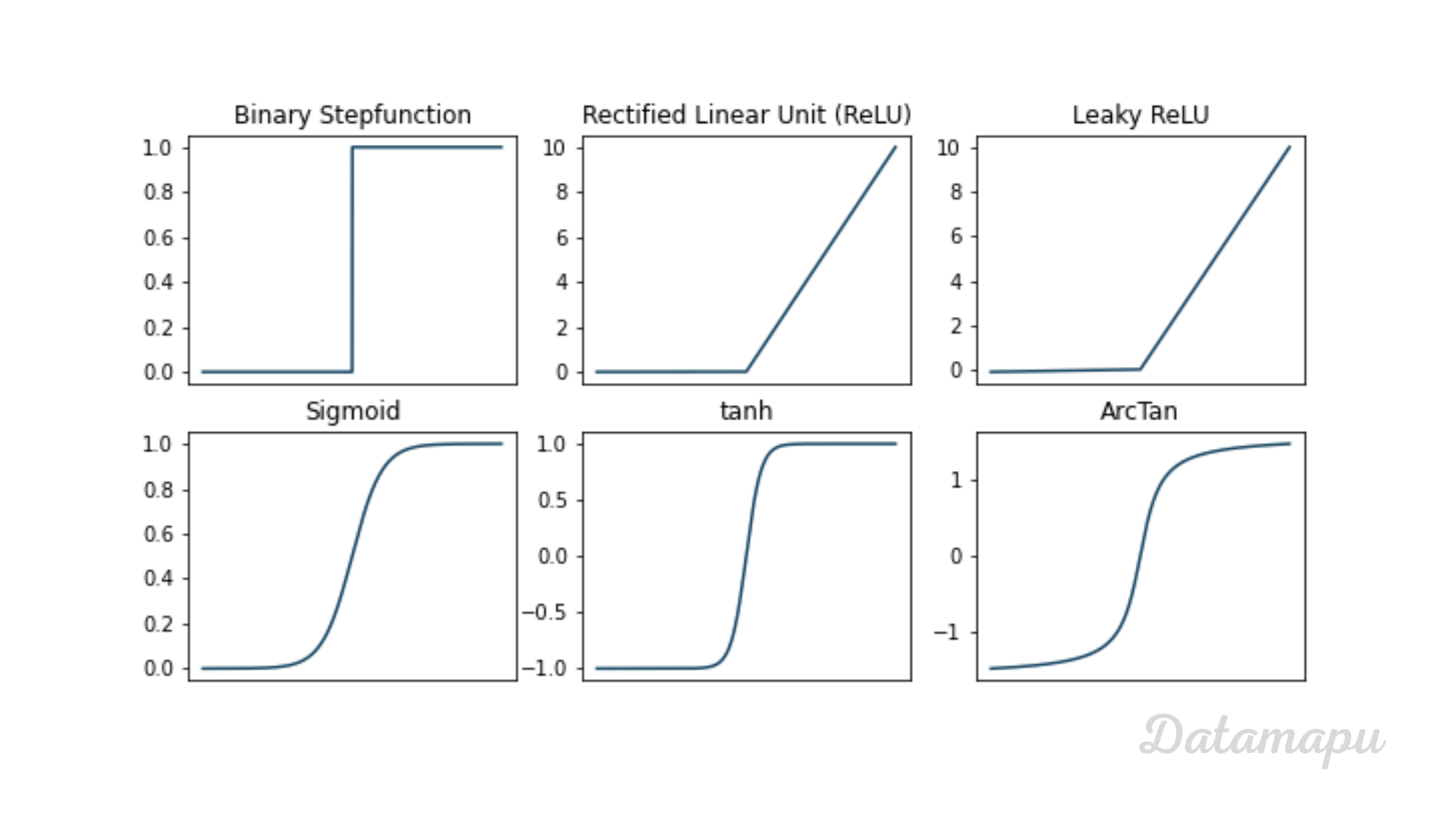ai_ml_dl Most common activation functions.

Neural Net

Multiple neurons can be joined together by connecting the output of one neuron with the input of another. This then results in a Neural Net as illustrated in the next plot. The connections are associated with weights that determine the “strength” of the connection. The weights - as mentioned earlier - are adjusted during training. Several neurons are aggregated into layers in a Neural Net. We distinguish between the input layer at the beginning, the output layer at the end, and the so-called hidden layers in between. In the following plot, the weights are drawn associated to layers. They are, however, different for each connection. That is $w_1$ to $w_4$ in this illustration are vectors, that contain the weights for each connection. The signal - that is the data - travels from the input to the output and passes through the hidden layers.

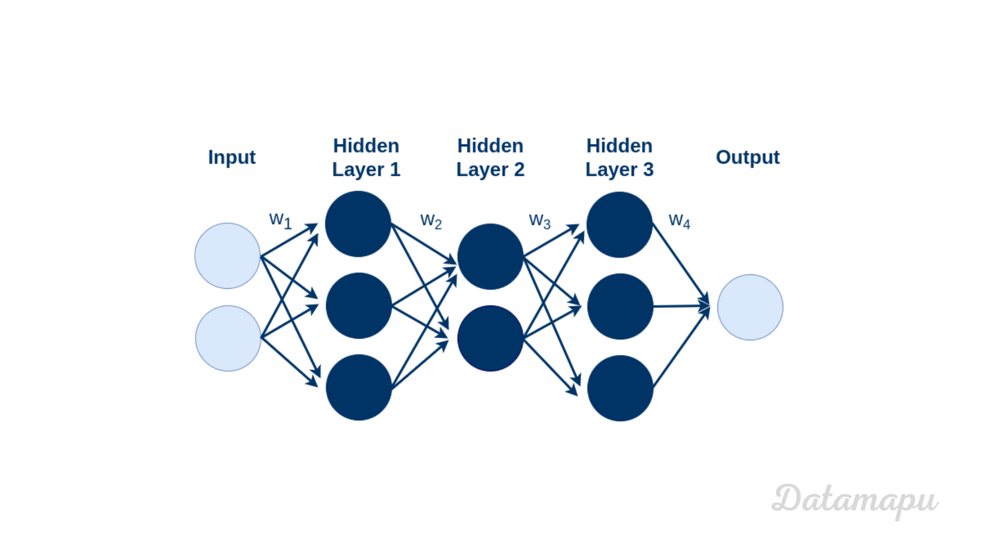ai_ml_dl Illustration of a Neural Net with 5 layers: 1 input layer, 3 hidden layers, and 1 output layer.

How does a Neural Net Learn?

Until now, we have seen how a neural net is organized. But we didn’t discuss yet, how the weights we use to calculate the output are determined. The process of finding the weights and bias is called training. This is the phase where the Neural Net is learning. Training a neural net is an iterative process. On a high level, the training process looks like this:

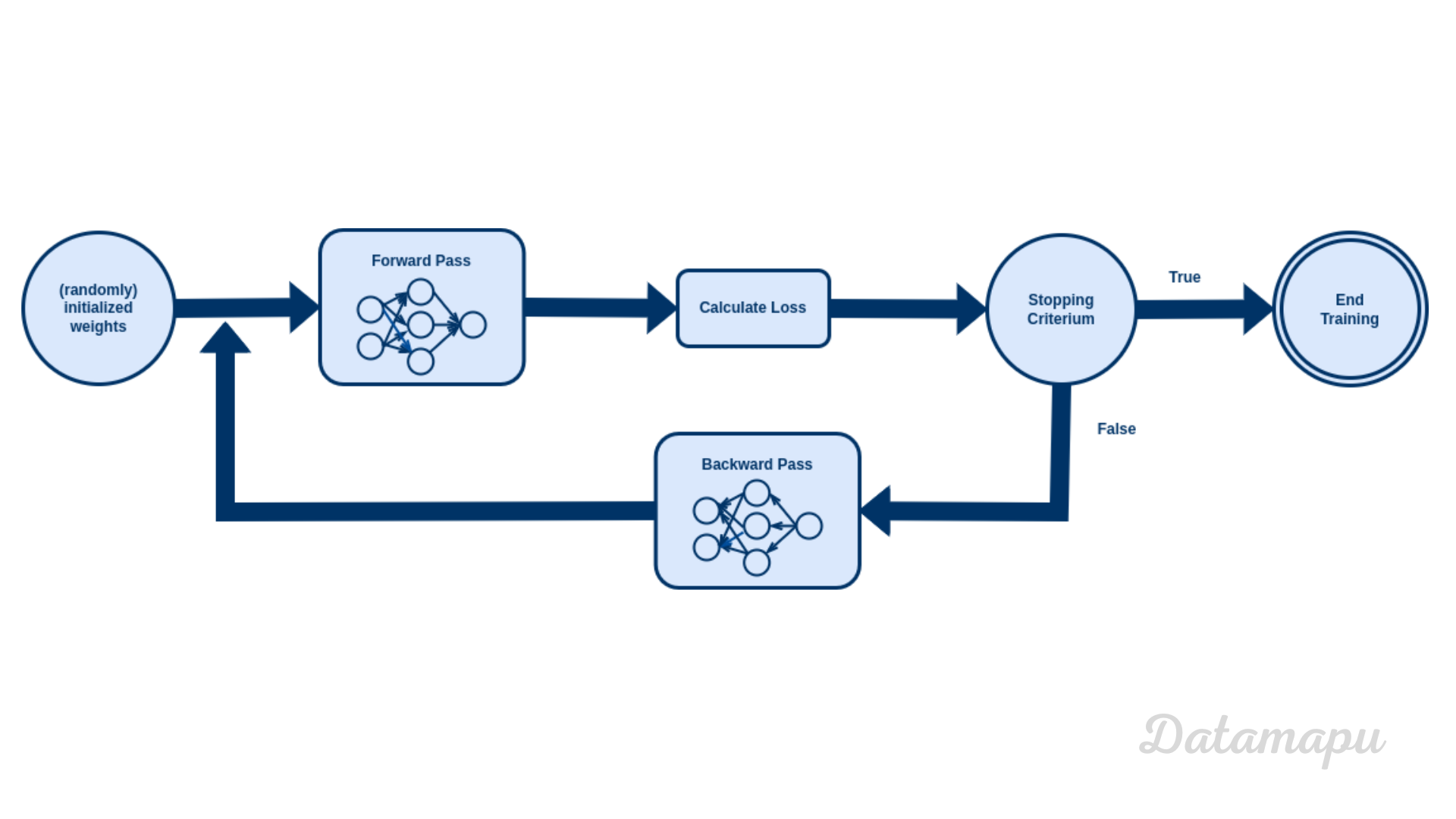ai_ml_dl Illustration of the learning process of a Neural Net.

Initially the weights are randomly generated.
Then the output of the Neural Net is calculated. This is the so-called forward pass.
Next the error between the output of the Neural Net and the true labels is calculated. This is the so-called loss. In the beginning - with random weights - the results of the Neural Net will usually not be good.
We check if the stopping criterium, which we defined is fullfilled.
If it is not fulfilled, the weights are adjusted in the so-called backward pass and the process starts again, i.e. we calculate the output (with the new weights), calculate the error compared to the true labels, which is then hopefully smaller than before - if the stopping criterion is not fulfilled, we adjust the weights, and so on. This is repeated until the stopping criterion is achieved, then the training ends.

In summary, this means the weights are iteratively adjusted and optimized, such that the error compared to the true values is minimized. But how can we achieve that the error gets smaller? To understand that, we have to focus on the loss. We have already mentioned the loss as the error between the Neural Net output and the true label. The function we use to calculate this error is the so-called loss function. The choice of the loss function depends on the problem you are considering. Typical loss functions are, the Mean Squared Error (MSE) for regression problems or cross-entropy for classification problems. The loss function is a function of the weights and biases. We want the loss to be as small as possible. In other words, this means that we want to minimize the loss function, with respect to the weights and the bias. That is, the goal for the training of a Neural Net is to adjust the weights, such that the loss function is minimized. There are different optimization techniques to approach this minimization problem. We will discuss the Gradient Descent, which is a standard algorithm for optimization.

Gradient Descent

As we just learned, we have to minimize the loss function in order to train a Neural Net. To do this, we can use different optimization techniques. We will take a look at one of these algorithms - the Gradient Descent. We will give a high-level overview. Here we illustrate the algorithm with a simplified example. The plot below shows the MSE as loss function $L$. We consider the one-dimensional case, which means we assume $L$ is a function of just one weight ($w$).

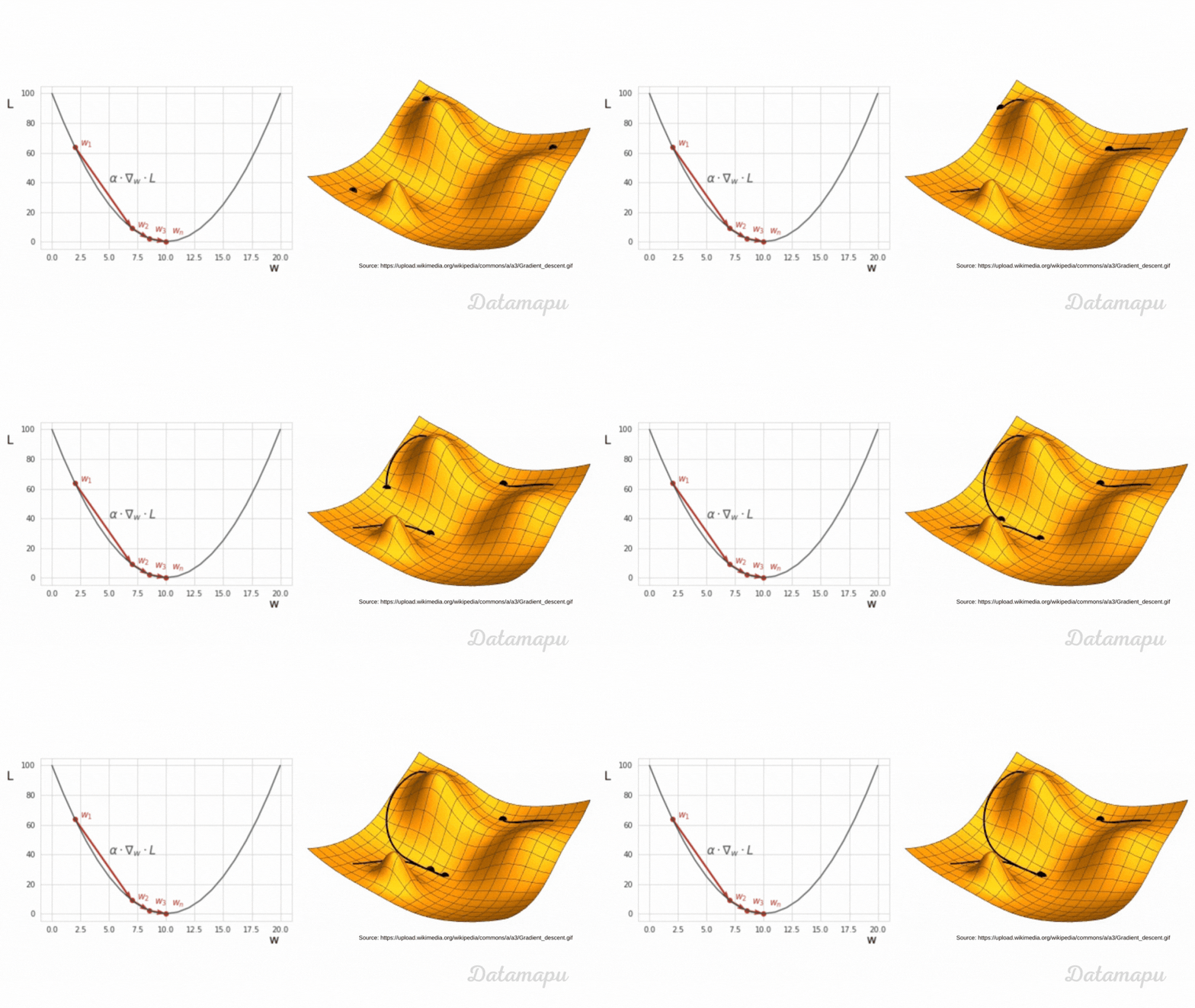ai_ml_dl Ilustration of Gradient Descent.

In Gradient Descent we start with some random value for the weight - here illustrated as $w_1$ - then we take small steps towards the minimum. To understand Gradient Descent we have to recall what the gradient is. The gradient of a function at a specific point is the direction of the steepest ascent. That is, if we want to find the minimum, we have to move in the opposite direction, that is in the direction of the negative of the gradient. This is, the direction of the steepest descent. How big this step is, is defined by the step size, a variable also called learning rate in the context of Machine Learning. This is a hyperparameter we have to define. Hyperparameters in Deep Learning have the same meaning as in classical Machine Learning. They are parameters whose values are used to control the learning process. In contrast to other parameters (such as e.g. weights), which are derived during training. When training a Neural Network we usually try different values. The calculation of the gradients is done by an algorithm called backpropagation. In this article we are not going into further detail. The choice of the learning rate influences the training. When the learning rate is very small, the training takes very long. If it is too large, we may miss the minimum. The weight of the next iteration is then updated by subtracting the learning rate multiplied by the gradient of the loss function at the previous weight. $$w_{i+1} = w_{i} - \alpha \cdot \nabla_{w_i} L(w_i) $$ In practice, a lot of variants of Gradient Descent exist. For example, classical Gradient Descent is applied to the entire dataset, before the weights are updated. This may take long if the dataset is large. A common variant is the mini-batch gradient descent, where data is passed in mini-batches through the network and the updates are calculated after each mini-batch.

How much Data do we need?

A question often asked is, how much data is actually necessary to use Deep Learning. Deep Learning is known to need a large amount of data, but what does that mean? Unfortunately, there is no answer to this, in the sense of giving a specific number of data points. The amount of data needed depends on different factors, such as e.g. the complexity of the task (what is not always known in advance), the quality of the available data, and the complexity of the network. In general, adding more data improves the performance, especially for complex tasks with large Neural Networks. However, if the data added is too similar to the data we already have, it will not give much new information to the Neural Network. If we don’t have much data available, but still want to use a complex Neural Net, we can can consider using a pretrained model (trained on a similar task) or data augmentation (especially when working with image data).

Summary

We discussed how Deep Learning is defined and learned that Deep Learning is a subset of Machine Learning. We introduced the structure of Neural Nets and learned that it consists of a set of connected neurons and that activation functions are used to introduce non-linearity into a Neural Net. We looked from a high-level perspective at how the learning process works and discussed that training a Neural Net is an iterative process, that aims to minimize the loss function. Lastly, we briefly discussed how much data is needed to apply Deep Learning. Unfortunately, there is no real answer to this question. How much data is needed depends on the problem we want to solve, the network, and the quality of the data. Generally speaking, we can say: the more data, the better.

If this blog is useful for you, please consider supporting.