Bias and Variance

January 1, 2024 - 8 minutes read - 1676 words

Introduction

In Machine Learning different error sources exist. Some errors cannot be avoided, for example, due to unknown variables in the system analyzed. These errors are called irreducible errors. On the other hand, reducible errors, are errors that can be reduced to improve the model’s skill. Bias and Variance are two of the latter. They are concepts used in supervised Machine Learning to evaluate the model’s output compared to the true values. For a Machine Learning model to be generalizable to new unseen data with high predictive skill, it is important that bias and variance are balanced.

Bias

The bias in a Machine Learning model is a systematic error in the predictions due to wrong assumptions during the modeling process. It describes the deviation from the model’s prediction to the true target data. Mathematically, the bias is defined as

$$Bias = E(\hat{Y}) - Y,$$

with $\hat{Y}$ the predictions produced by the Machine Learning model and $Y$ the true target values. That is, the bias is the difference between the expected model predictions and the true values. A bias results from assumptions that are made of the underlying data. Since every Machine Learning model is based on some assumptions, all models underly a certain bias. A low bias means fewer assumptions were made and the model fits the data well. A high bias can be introduced by using too simplified assumptions about the mapping that is supposed to be modeled, e.g. using a model that is too simple. In this case, the model is not able to capture the underlying pattern of the data. This is also known as underfitting.

Possibilities to reduce the Bias

In general, a low bias is desirable. There is, however, no recipe for how to reduce it. The following methods can be tried.

Select a more complex model architecture. If the selected model is too simple compared to the underlying data, the bias will always be high. For example, if a linear model is used to model a non-linear relationship, the model will never be able to capture the underlying pattern, no matter how long and with how much data is trained.

Increase the number of input features. More complexity can not only be introduced by the model structure itself but also by using more input features. The additional features can help to identify the modeled relationship.

Gather more training data. A larger training dataset can help to learn the underlying pattern between input features and target data.

Decrease regularization. Regularization techniques are used to prevent overfitting and make the model more generalizable. This is useful if the model shows high variance, as we will see in the next section. However, if the bias is high reducing the regularization may help.

Variance

Variance is a term from statistics, which measures the spread of a variable around its mean. In Machine Learning it describes the change in the predictions when different subsets are used for training, or in other words the variability of the model’s prediction. Mathematically the variance is described as the expected value of the square of the difference between the predicted values and the expected value of the predictions

$$Variance = E[(\hat{Y} - E[\hat{Y}])^2],$$

with $\hat{Y}$ the predictions produced by the Machine Learning model and $Y$ the true target values. Low variance means that the variability between the training on different subsets is low. That is the model is less sensitive to changes in the training data and able to generalize to unseen data equally well independently of the data subset it was trained on. On the other hand high variance means that the model is highly sensitive to the training data and the model results differ depending on the selected subset. High variance implies that the model fits very well to the training data, but is not able to generalize to new data. This phenomenon is called overfitting. High variance can result from a complex model with a large set of features.

Possibilities to reduce the Variance

To make the model generalizable to new data, a low variance is desirable. As for the bias, there is no recipe to achieve this. The following methods may help to reduce the variance.

Select a less complex model. High variance often results from a model that is too complex, that fits the specific training data sample too well and by doing that oversees the general pattern.

Use cross validation. In cross validation, the training data is split into different subsets that are used to train the model. Tuning the hyperparameters on different subsets can make the model more stable and reduce the variance.

Select relevant features. Analog to reducing the bias by increasing the number of features, we can try to reduce the variance by removing features and with that reduce the complexity of the model.

Use regularization. Regularization adds an extra term to the loss function, which is used to weigh features by their importance.

Use ensemble models. In Ensemble learning, multiple models are used and aggregated into one single prediction. Different types of ensemble models exist, Bagging is especially suited to reduce the variance.

The following table shows and summarizes all possible combinations of Bias and Variance.

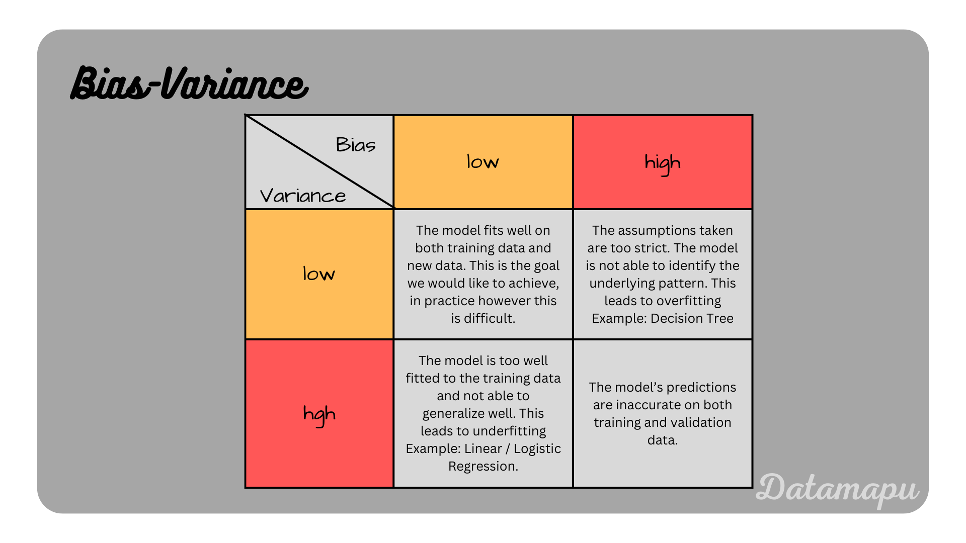Overview about the combinations of bias and variance.

The effect of Bias and Variance is often illustrated using a dartboard as shown in the following plot.

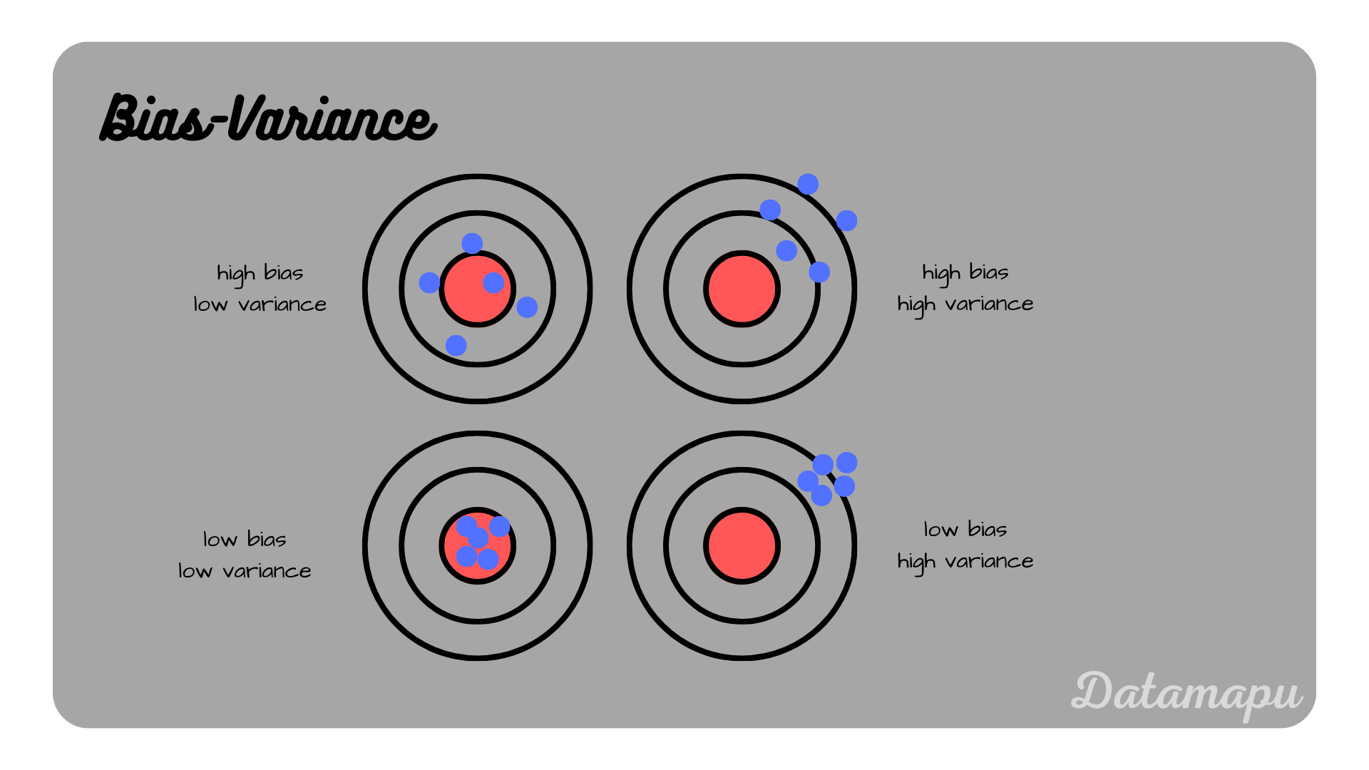Illustration of the combinations of bias and variance.

Bias-Variance Tradeoff

Concluding the above derivations, it is in general desirable to achieve a low bias as well as a low variance. This is however difficult. Intuitively this is clear because a model cannot be simple and complex at the same time. Mathematically, the bias and the variance are part of the total error of a Machine Learning model. Let $Y$ be the true values and $\hat{Y}$ the model’s estimates with $Y = \hat{Y} + \epsilon$ and $\epsilon$ a normally distributed error with mean $0$ and standard deviation $\sigma$. The predictions $\hat{Y}$ depend on the dataset the model has been trained on, while the true values $Y$ are independent of the specific dataset. The expected (squared) error, that is aimed to be minimized can then be written as

$$E[(Y - \hat{Y})^2] = E[Y^2 - 2Y\hat{Y} + \hat{Y}^2].$$

Because of the linearity of the expected value this equal to

$$E[(Y - \hat{Y})^2] = E[Y^2] - 2E[Y\hat{Y}] + E[\hat{Y}^2]. (1)$$

Let’s consider these three terms individually. We can reformulate $E[Y^2]$ as follows

$$E[Y^2] = E[(\hat{Y} + \epsilon)^2] = E[Y^2] + 2E[Y\epsilon] + E[\epsilon^2].$$

Since the true values $Y$ are independent of the dataset, this is equal to

$$E[Y^2] = Y^2 + 2YE[\epsilon] + E[\epsilon^2].$$

We can use the following formula of the variance for a variable $X$

$$Var[X] = E[(X - E[X])^2]$$

and reformulate it as

$$Var[X] = E[X^2 - 2XE[X] + E[X]^2]$$ $$Var[X] = E[X^2] - 2E[X]E[X] + E[X]^2$$ $$Var[X] = E[X^2] - E[X]^2$$

to rewrite this equation. Since we assumed $\epsilon$ to have mean $0$ and standard deviation $\sigma$ the term simplifies to

$$E[Y^2] = Y^2 + 2YE[\epsilon] + Var[\epsilon] + E[\epsilon^2] = Y^2 + \sigma^2. (2)$$

Using the equation for the variance, the last term of equation (1) can be written as

$$E[\hat{Y}^2] = E[\hat{Y}^2] - E[\hat{Y}]^2 + E[\hat{Y}]^2 = Var[\hat{Y}] + E[\hat{Y}]^2. (3)$$

Putting (2) and (3) back into equation (1) and using the indepence of $Y$ of the dataset, leads to

$$E[(Y - \hat{Y})^2)] = Y^2 + \sigma^2 - 2YE[\hat{Y}] + Var[\hat{Y}] + E[\hat{Y}]^2.$$

This can be written as

$$E[(Y - \hat{Y})^2] = (Y - E[\hat{Y}])^2 + Var[\hat{Y}] + \sigma^2.$$

In other words the total error in a Machine Learning model is

$$E[(Y - \hat{Y})^2] = Bias^2 + Variance + \sigma^2,$$

with $\sigma$ being the irreducible error. The total error of a Machine Learning Model is thus composed of the Bias, the Variance, and the irreducible error. The difficulty of minimizing both bias and variance to find a good balance such that the model does not overfit and not underfit is known as the Bias-Variance Tradeoff. It can be illustrated as follows.

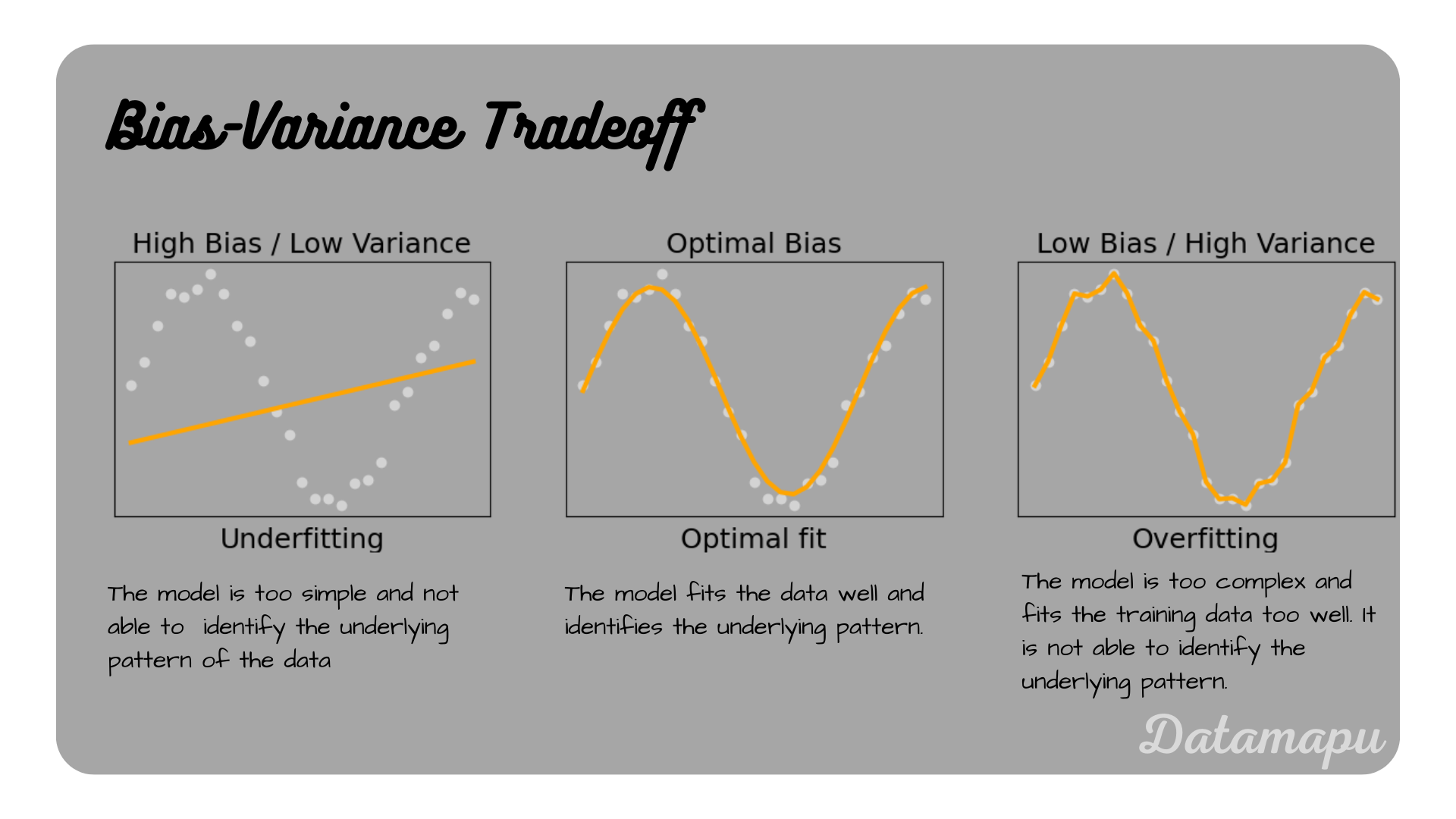bias and variance Underfitting and Overfitting illustrated for a regression problem.

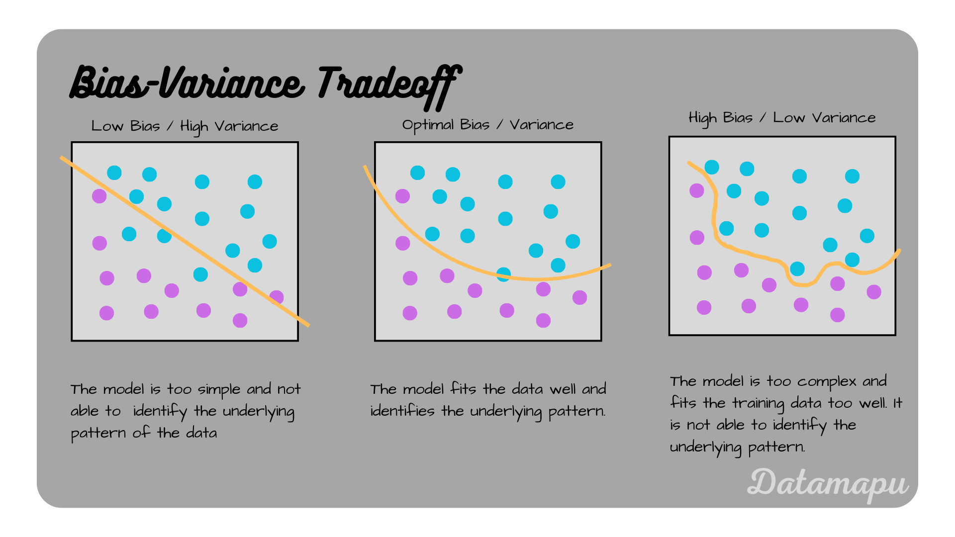bias and variance Underfitting and overfitting illustrated for a classification problem.

The relationship between the general error, Bias, and Variance can be illustrated as follows

bias and variance https://commons.wikimedia.org/w/index.php?curid=105307219 (Von Bigbossfarin - Eigenes Werk, CC0)

Example

To illustrate the modelling of simple to complex models, we consider an example of a polynomial function, which is modeled by polynoms of different degrees.

 1
 2
 3
 4
 5
 6
 7
 8
 9
10
11
12
13
14
15
16
17
18
19
20
21
22
23
24
25
26
27
28
import numpy as np

fig, ax = plt.subplots(3, 2, figsize=(12,16))
np.random.seed(42)
x = np.arange(0,30,1)
noise = np.random.normal(0, 500,x.shape[0])
a0 = 20
a1 = 0.3
a2 = -25
a3 = 1.1
y = a0 + a1*x + a2*x**2 + a3*x*x*x

# training data
y1 = y + noise

# models
# 1. linear
model1 = np.poly1d(np.polyfit(x, y1, 1))
# 2. quadratic
model2 = np.poly1d(np.polyfit(x, y1, 2))
# 3. cubic
model3 = np.poly1d(np.polyfit(x, y1, 3))
# 4. degree 10
model4 = np.poly1d(np.polyfit(x, y1, 10))
# 5. degree 15
model5 = np.poly1d(np.polyfit(x, y1, 15))
# 6. degree 20
model6 = np.poly1d(np.polyfit(x, y1, 20))

Plotting the different models against the “true model” $y = 20 + 0.3x - 25x^2 + 1.1 x^3$ shows how simple models as the linear one show a high bias and complex models as the one of degree $20$ show a high variance. The cubic model fits the true model best.

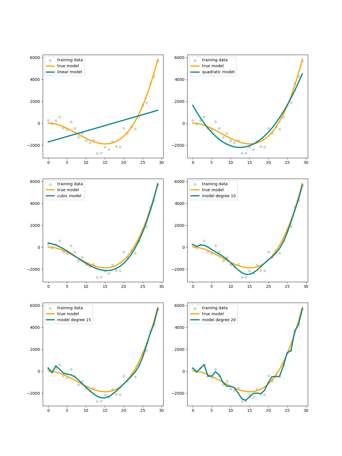bias and variance Example for polynomial models of different degrees.

Summary

Bias and Variance are different types of errors in Machine Learning. Both high bias and high variance mean that a model is not able to understand the underlying pattern of the data and is therefore not able to generalize to new unseen data. In practice, it is important to balance bias and variance to achieve a good model.