Metrics for Classification Problems

Classification Problems

Supervised Machine Learning projects can be divided into regression and classification problems. In regression problems, we predict a continuous variable (e.g. temperature), while in classification, we classify the data into discrete classes (e.g. classify cat and dog images). A subset of classification problems is the so-called binary classification, where only two classes are considered. An example of this is classifying e-mails as spam and no-spam or cat images versus dog images. When we consider more than two classes, we speak of multi-class classification. An example of this is the MNIST dataset, where images of handwritten digits are classified, i.e. we have 10 different classes. Depending on the problem we consider, we need different metrics to evaluate our Machine Learning model. Within each of these two types of Machine Learning problems, we have to choose which of the metrics fits our needs best. This post will give an overview of the most common metrics for binary classification problems, what they mean, and when to use them.

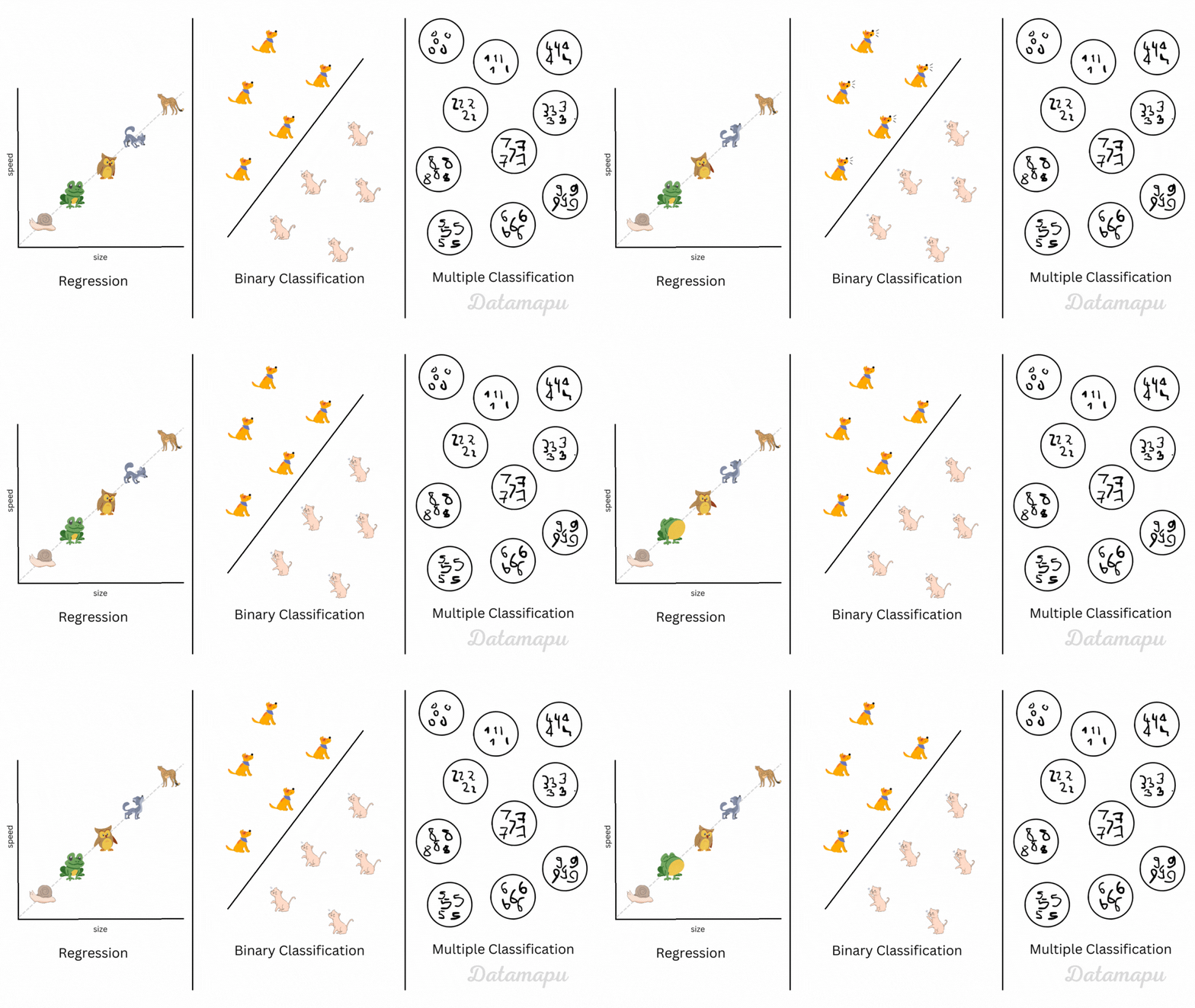Regression, binary classification and multiple classifiction illustrated.

Confusion Matrix

A good way to start evaluating a classification problem is the so-called confusion matrix. It gives an overview of how many predictions were correct and how many were not for each class. Let’s imagine we want to classify cat and dog images and our model gives the following result on 10 test images.

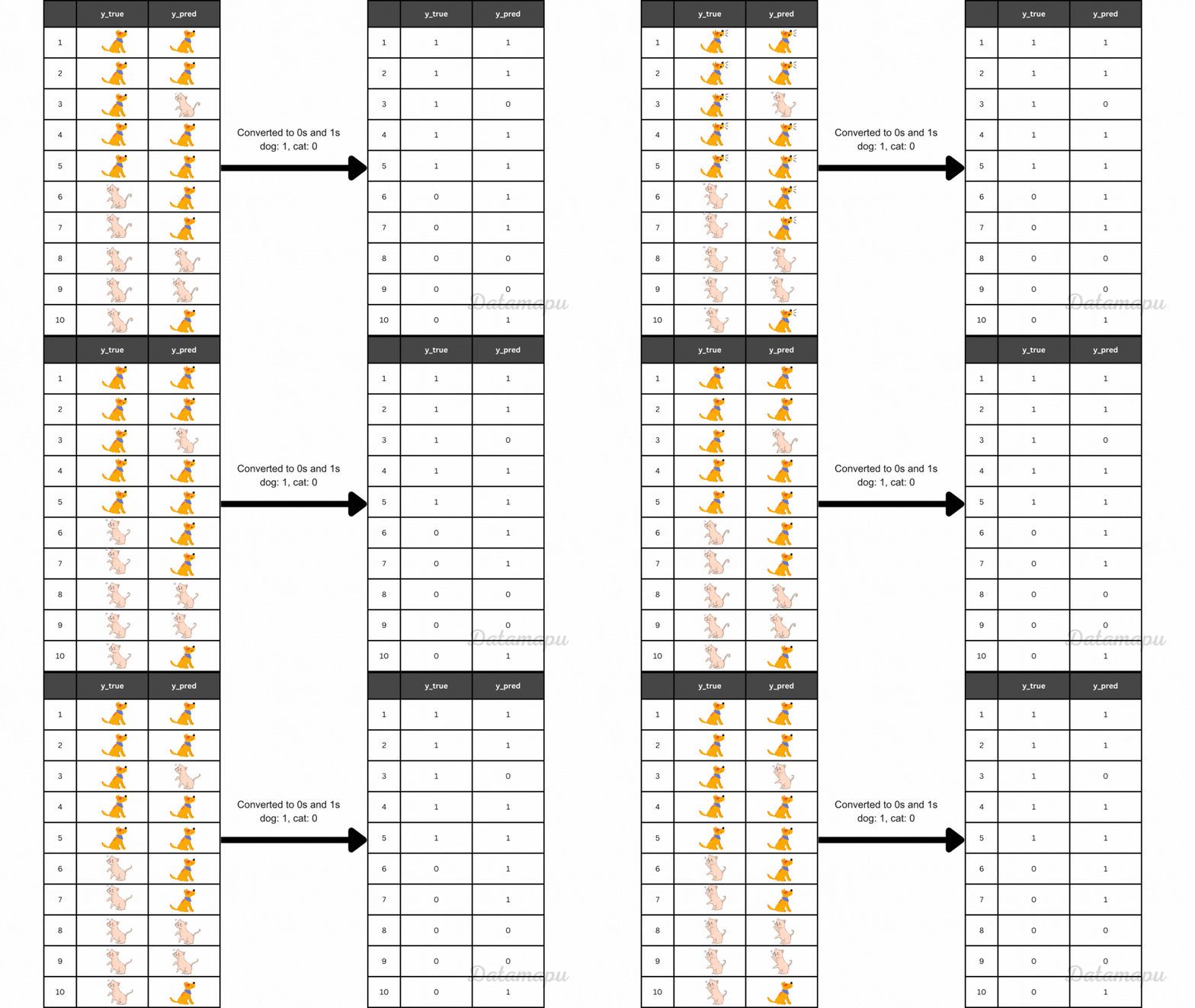Example true and predicted values converted to 0s and 1s.

From this table, we can see when our model was correct and when not. The confusion matrix is a way to illustrate these results more clearly. We can use the scikit-learn package to display the confusion matrix in Python.

We can then display the confusion matrix as follows:

1
2
3
4
5

from sklearn.metrics import confusion_matrix, ConfusionMatrixDisplay
cm = confusion_matrix(y_true, y_pred)
disp = ConfusionMatrixDisplay(confusion_matrix=cm,
                              display_labels=["cat", "dog"])
disp.plot();

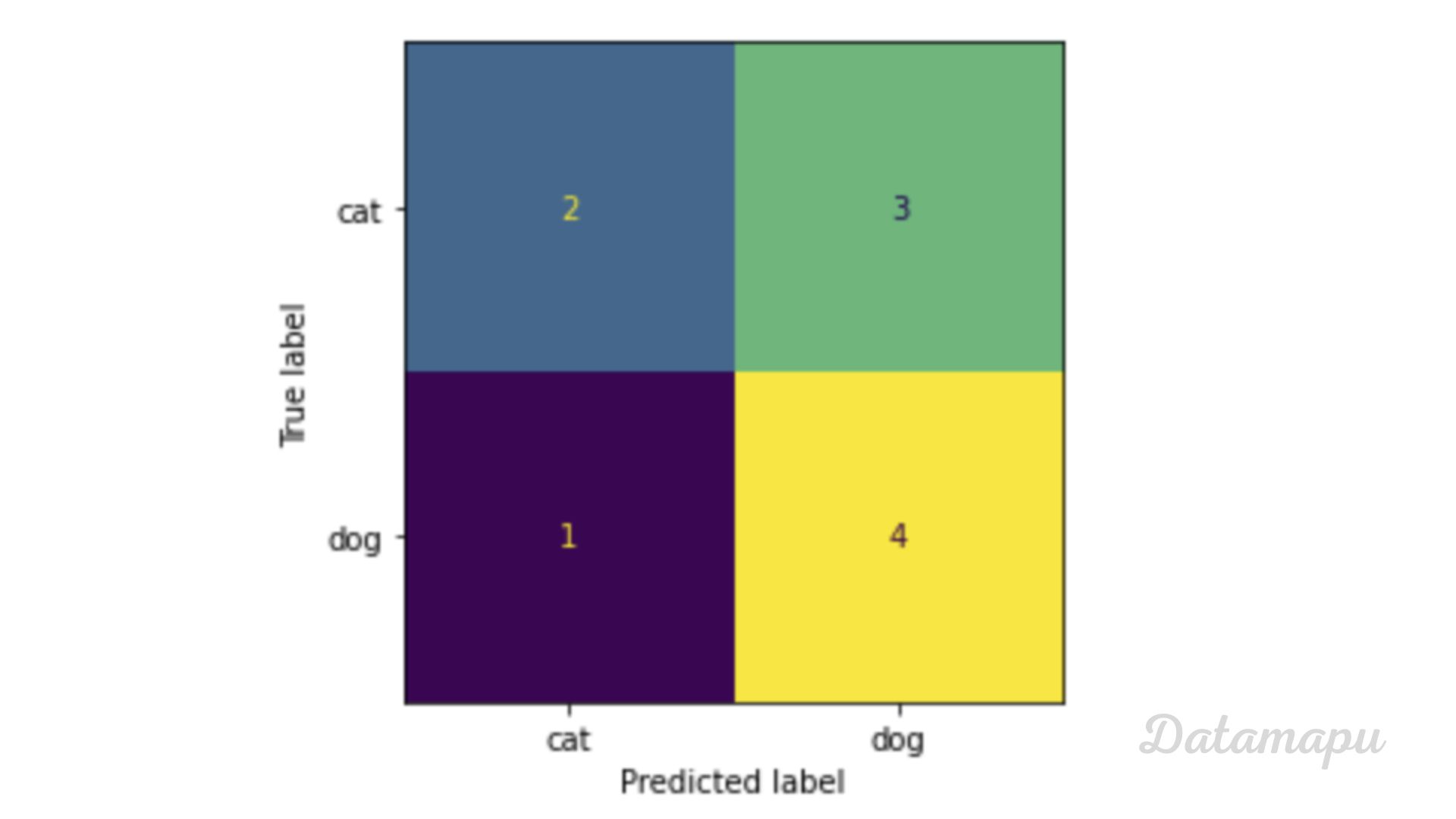Confusion matrix example.

The confusion matrix shows the predicted labels versus the true labels, and the numbers in the matrix give the number of images that were predicted for each case. The first column, first row of the matrix (cat - cat) shows how many results predicted a cat and the real image was also a cat. The first column, second row (cat-dog) shows how many results predicted a cat, but the true label was a dog and so on. Note, that this not only divides into correct and incorrect, but also in the type of error we make. There are four possible outcomes:

• TP (True Positive): The prediction is a dog (positive) and the true image is also a dog (positive)
• FN (False Negative): The prediction is a cat (negative), but the true image is a dog (positive)
• FP (False Positive): The prediction is a dog (positive), but the true image is a cat (negative)
• TN (True Negative): The prediction is a cat (negative) and the true image is a cat (negative).

More general this looks like this. 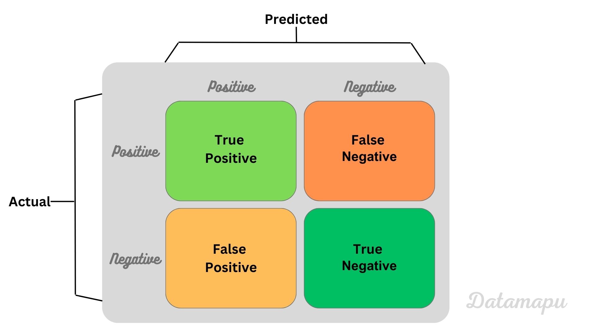Confusion matrix.

Metrics

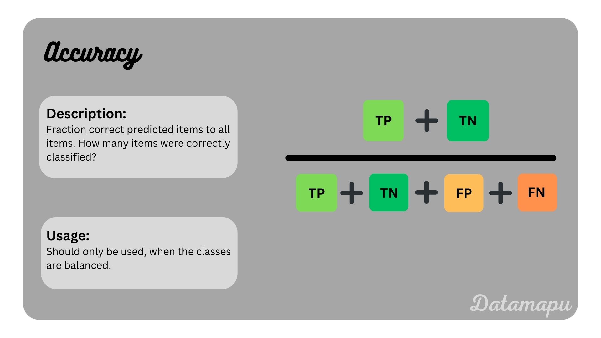
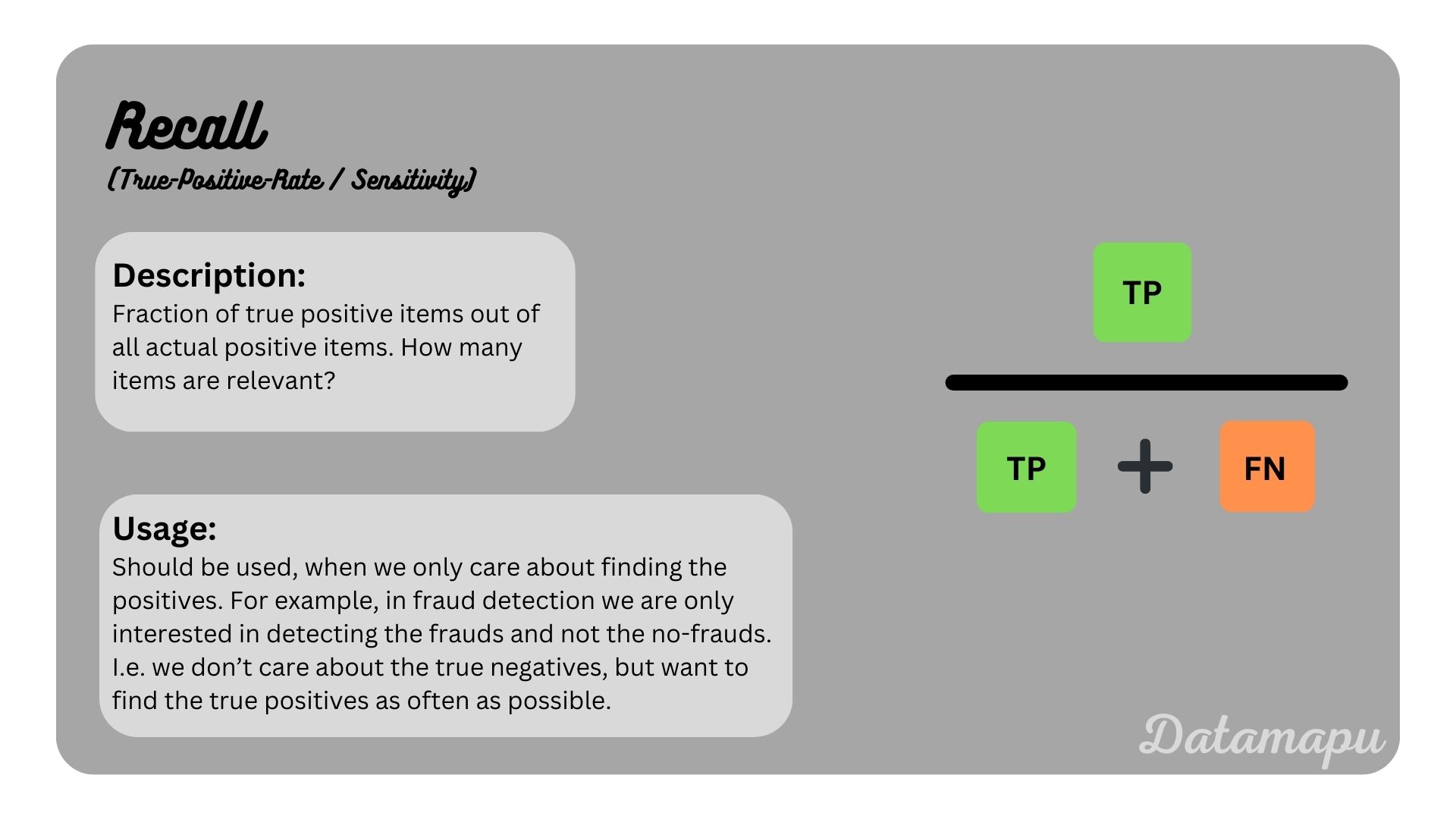
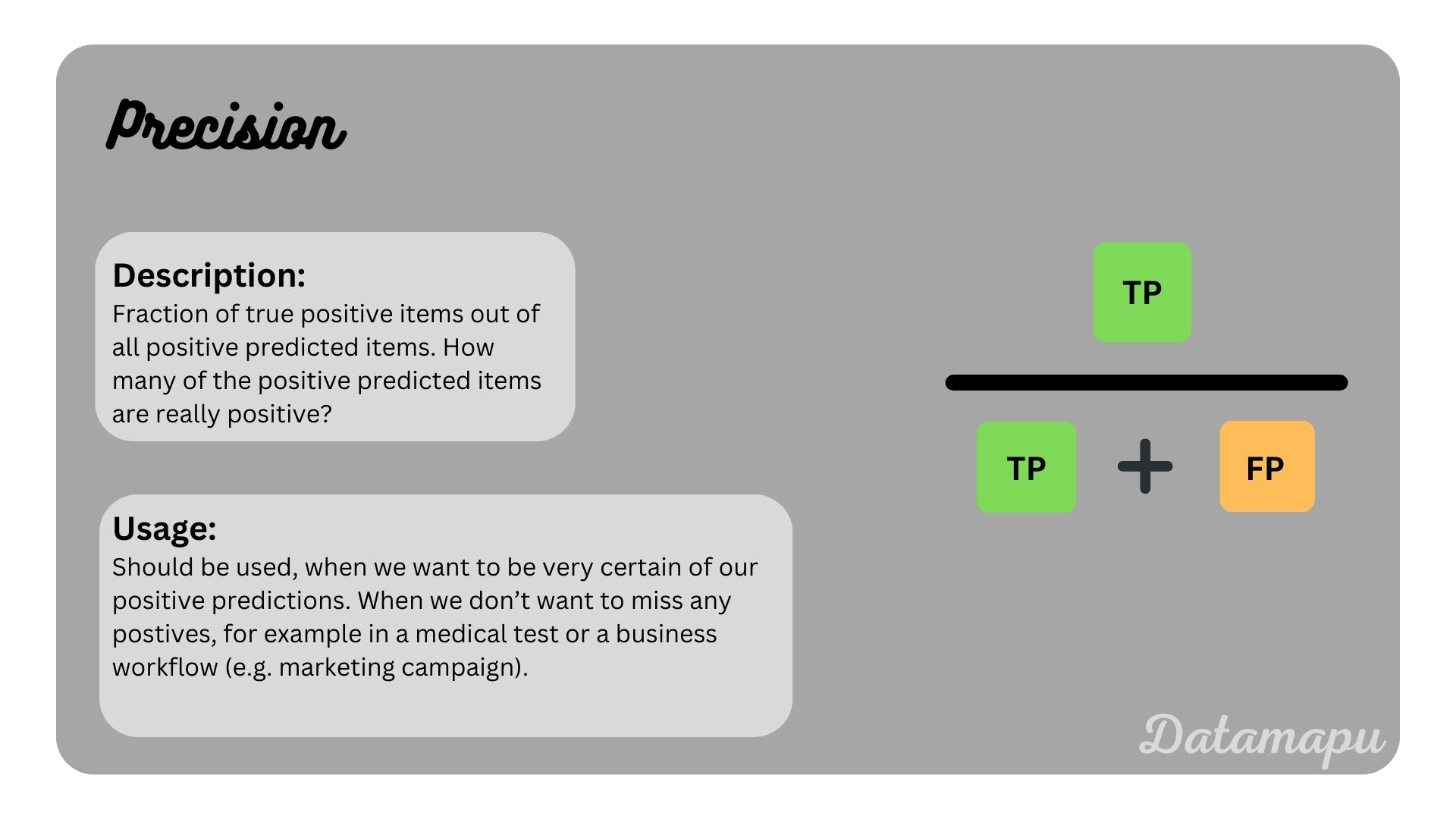
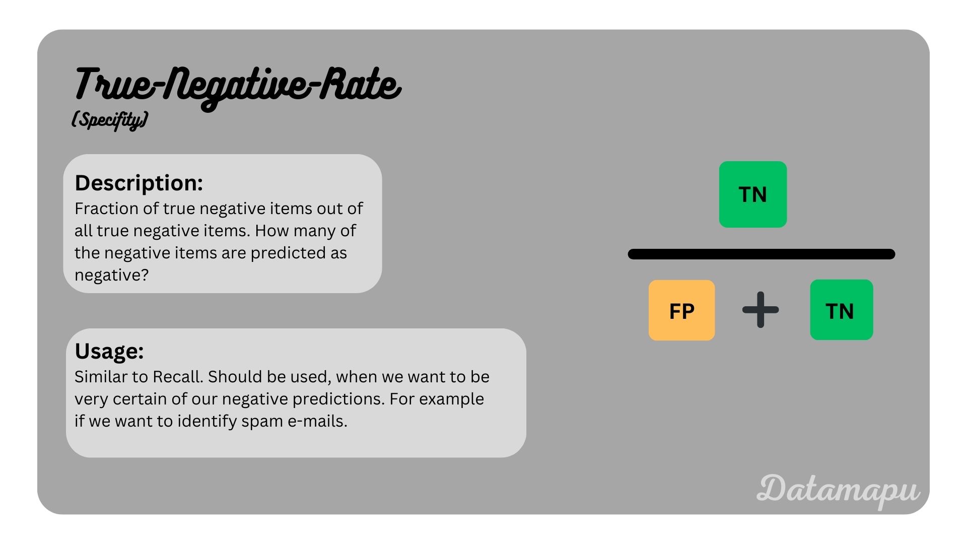
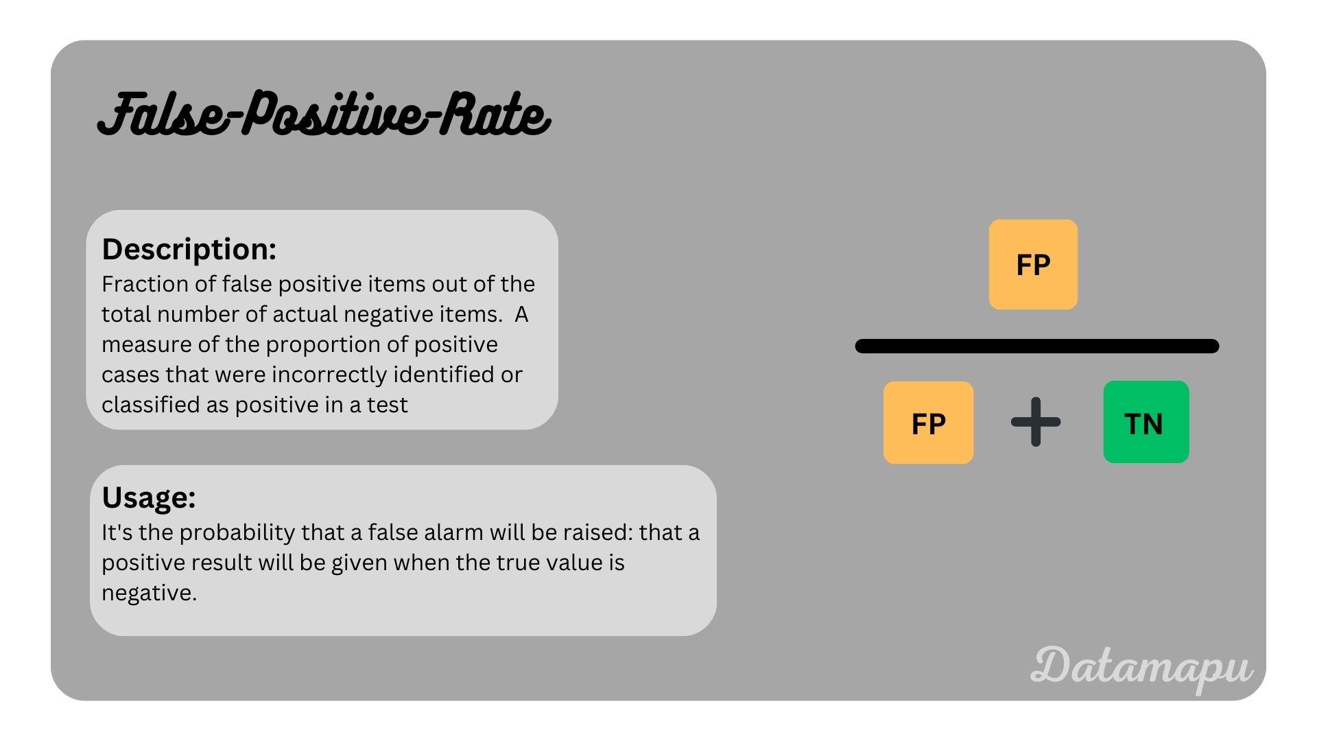
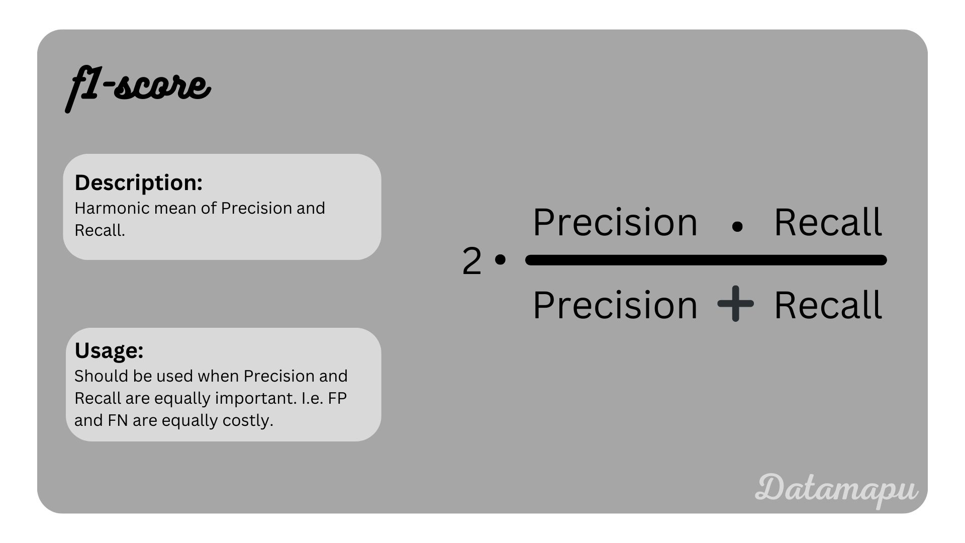
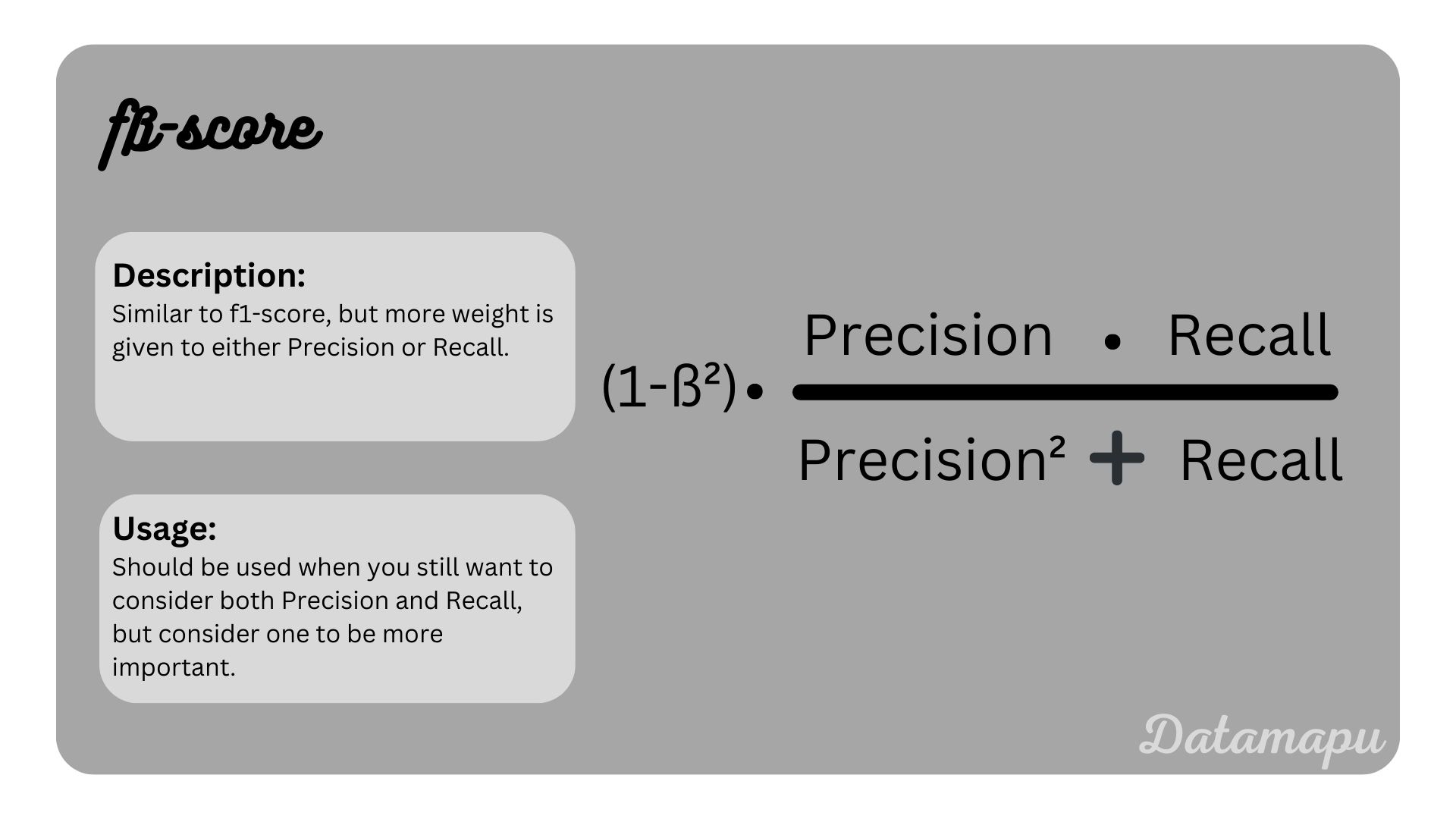
With the above concepts of TP, FN, FP, and TN we can define several metrics that evaluate binary classification problems in different aspects. Let’s have a look at the most common metrics for binary classification problems, how to calculate them and when to use them.

Classification Threshold

To classify into positive and negative predictions, we need to define a threshold. Predictions below this threshold are classified as 0 (cat) and predictions above are classified as 1 (dog). By default this value is 0.5, but we can change it. When we change the threshold, the number of TP, FN, FP, and TN change and with that the above defined metrics. In the following image five different thresholds are illustrated for our example of classifying dog and cat images. The resulting change in Recall / True-Positive-Rate (TPR) and False-Positive-Rate (FPR) is shown.

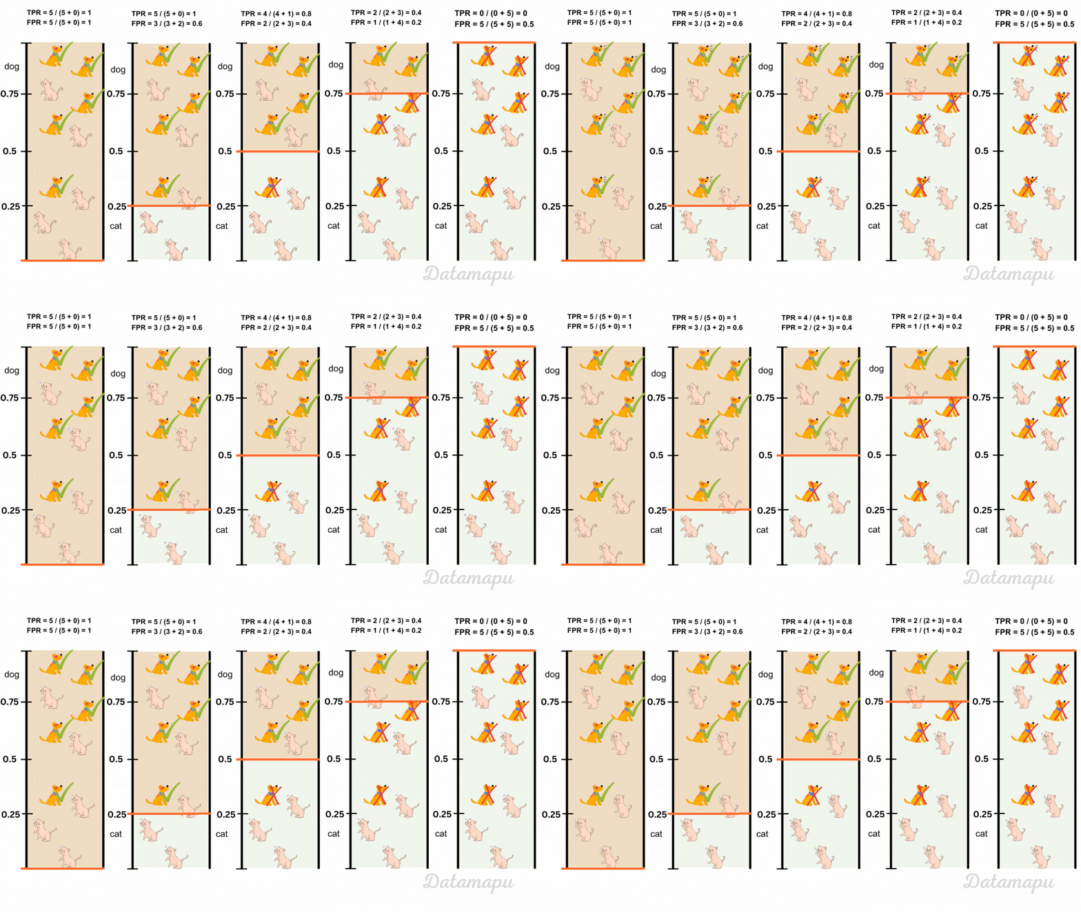The change of Recall / True-Positive-Rate (TPR) and False-Positive-Rate (FPR) with the change of the classification threshold.

When we compare Recall / True-Positive-Rate and False-Positive-Rate for different thresholds and plot their values against each other, we get the Receiver-Operator-Characteristics (ROC) Curve. The ROC-Curve can help us to fnd a suited threshold for our task.

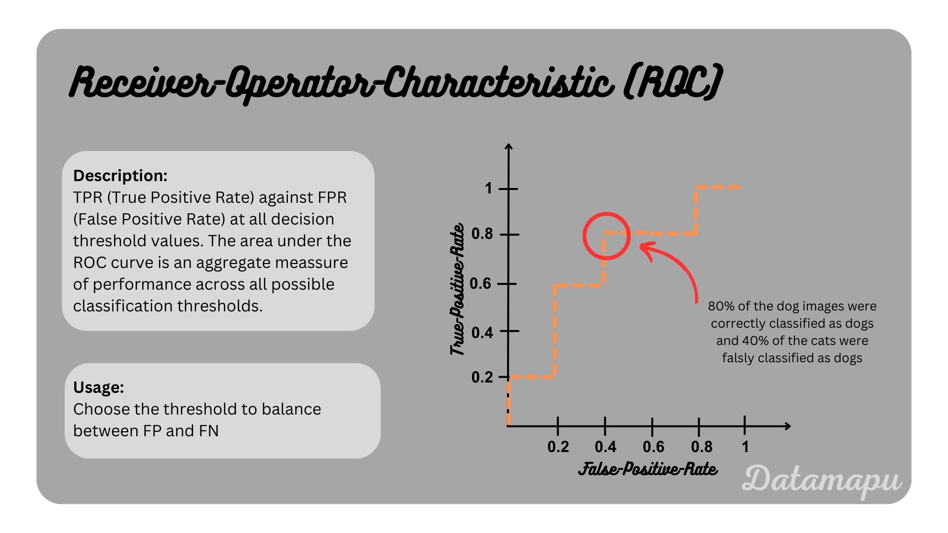
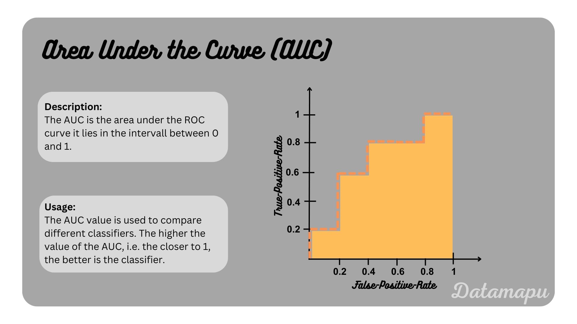
Using the ROC curve we can compare different classifiers. The higher the curve, the better a classifier. If the ROC curve was the diagonal, this would equal the classifer to make random guesses. The Area Under the Curve (AUC) is used to meassure this value. It lies between 0 and 1. The closer it is to 1, the better the classifier. In the case of the diagonal, the AUC would equal 0.5.

Example

In Python you can calculate all these metrics - for binary and multiple classification - using the sklearn metrics module, e.g. accuracy can be calculated as follows:

1
2

from sklearn.metrics import accuracy_score
acc = accuracy_score(y_true, y_pred)

For the above example of classifying cat and dog images, we achieve an accuracy of 6/10 = 0.6, because 6 images (4 dogs and 2 cats) out of 10 are correctly classified.

Summary

Binary classification is a specific case of classification problems, where the data is divided into two classes. Depending on the focus of the project the classifier can be optimized towards specific metrics. The above defined metrics are the most common metrics for binary classification. If none of these suite your purpose you can of course define your own custom metric to evaluate your classifier. Further the threshold towards the data is classified can be changed in order to optimize towards a certain metric. All the above defined metrics can be generalized for multiple classification.

If this blog is useful for you, please consider supporting.

• Data Science
• Machine Learning
• Classification
• Metrics