Feature Selection Methods

December 11, 2023 - 8 minutes read - 1624 words

Introduction

Feature Selection is the process of determining the most suitable subset of the total number of available features for modeling. It helps to understand which features contribute most to the target data. This is usefull to

Improve Model Performance. Redundant and irrelevant features may be misleading for the model. Additionally, if the feature space is too large compared to the sample size. This is called the curse of dimensionality and may reduce the model’s performance.
Reduce Overfitting. Feature selection can reduce overfitting in different ways. Removing features that are not useful for the model, reduces the noise in the data which may irritate the model. If highly correlated features are included the model may give them more weight, which may lead to overfitting. By removing highly correlated features the redundancy is reduced.
Reduce Training Time. The more data, the longer the training takes. If we reduce the feature space, the training time will be reduced and more efficient.
Increase Explainability. In general more simple models are easier to interpret. That is not only true for the model structure, but also for the number of input features included. In a model with fewer input features it is easier to analyze their influence on the target data.

Feature Selection Methods

In this post, we will only discuss feature selection methods for supervised machine learning algorithms, that is for data where labels are available. Three types of feature selection methods are differentiated: wrapper methods (e.g. forward, backward, and stepwise selection), filter methods (e.g. Pearson’s correlation coefficient, LDA, ANOVA, and chi square), and embedded methods (e.g. Lasso regulation and Decision Tree). We will present a high level overview of each of the methods below.

Wrapper Methods

Wrapper methods are based on training a machine learning model on different subsets of the feature space. New features are systematically included or excluded and based on the results compared to the previous model it is decided whether the new feature is included or not. Different models need to be trained and evaluated to identify the optimal set of features, which means these models are computationally expensive. The three most common wrapper methods are

Forward Selection. In forward selection, we start with one single feature and iteratively increase the number of features. The model is fitted with each of the possible features individually. That is, if $m$ features are considered, $m$ models are fitted. The feature resulting in the best performing model is chosen. In the next step, this first feature remains fixed and subsequently, all the other features are individually added to the model. That is in this second step $m-1$ models are fitted. The feature that improves the model with only one feature the most is selected. This procedure is continued until there is no further improvement.
Backward Selection. Backward selection is also an iterative method. In backward selection, however, we start with the full set of possible features and fit a model with all the features included. In the next step, one of the features is eliminated and the model is retrained with $m-1$ features. This is repeated for all features, resulting in $m$ models. The results are compared to the model including all features and the model that improves the most is chosen and accordingly the feature space is reduced by one. This procedure is continued until there is no further improvement.
Exaustive Feature Selection. In this method, all possible subsets of features are used and modeled. The resulting models are compared and the features used in the best model are chosen. This method is even more computationally expensive than the other two.

Filter Methods

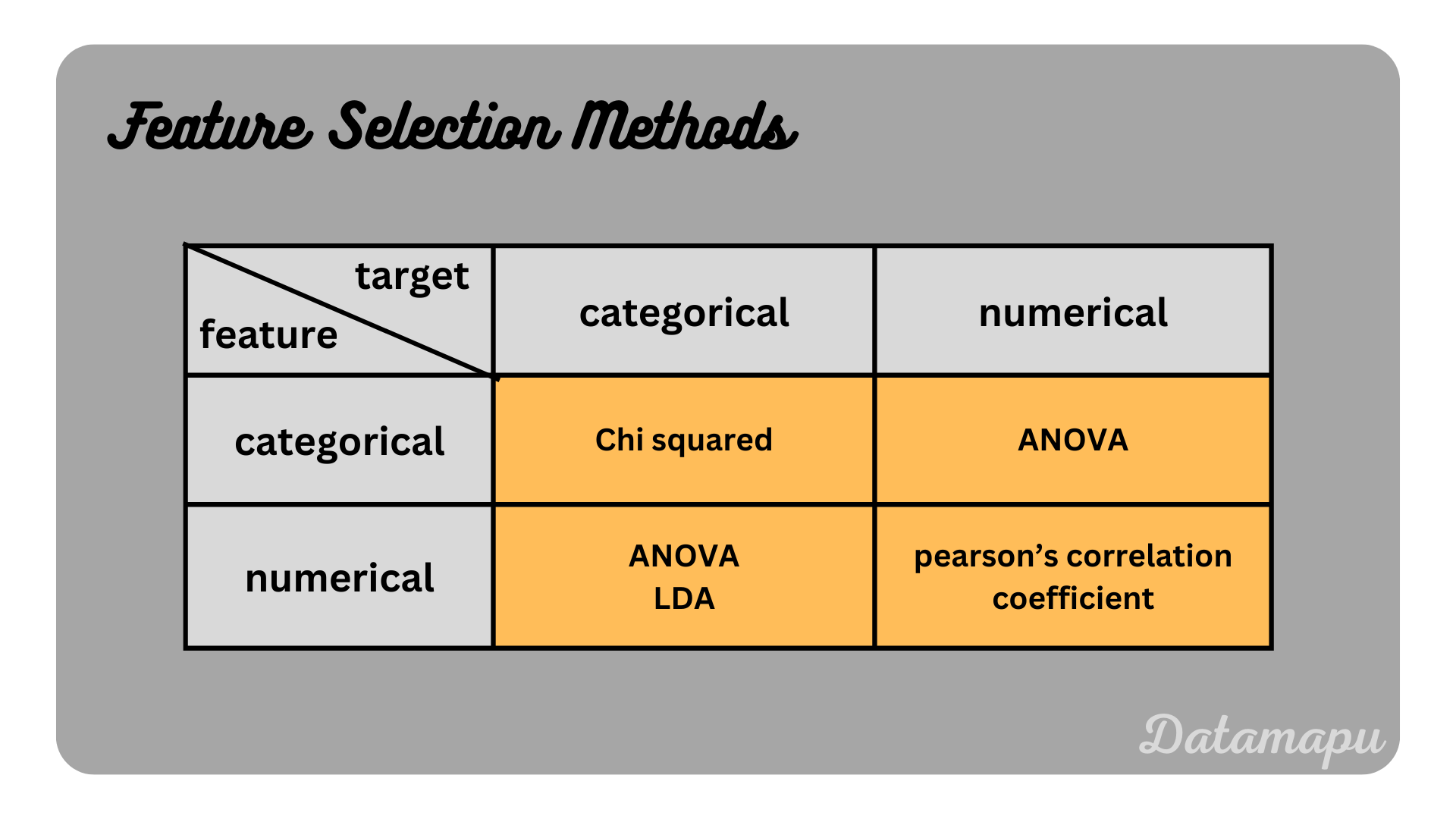
In contrast to wrapper methods filter methods do not depend on a Machine Learning model but are applied when the data is preprocessed, i.e. before the training starts. Statistical relationships between the features and the target are used to identify the most significant features. Filter methods are computationally lighter than wrapper methods, but the selection is more subjective as there is no exact rule for the features that are selected. Which exact method is suitable also depends on whether the input features and target data are numerical or categorical.

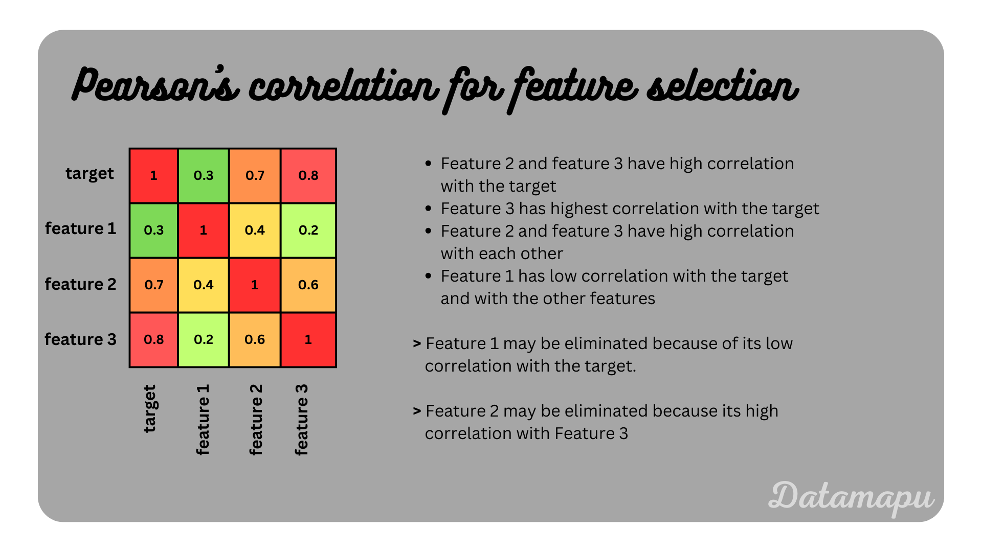
Pearson’s Correlation Coefficient. Pearson’s correlation coefficient is suitable for numerical input features and target data. The correlation coefficient measures the linear relationship between two variables. It takes values between $-1$ and $1$, with $-1$ meaning perfectly negatively correlated, $1$ perfectly positively correlated, and $0$ meaning that the variables are not correlated. To select the most important features the correlation between each feature and the target variable is calculated. Then features with the highest absolute correlations are selected for modelling. This can be done by setting a threshold of e.g. $\pm0.5$ or $\pm0.6$ and features with a higher correlation with the target are used. The correlation coefficient can also be used to find multicollinearity within the features, which may disturb the training and should be removed. If for example, two features have a high correlation with the target variable but also have a high correlation with each other only one should be used.

Illustration of feature selection using pearson’s correlation coefficient.

Linear Discriminant Analysis (LDA). LDA is a supervised machine learning algorithm for classification problems that is used to reduce dimensionality. As we consider classification problems, the target data needs to be categorical. LDA aims to find a linear combination of the features such that these categories are maximally separated. Loosly speaking this is done by projecting the data onto a coordinate system, such that the distance of the means of the classes is maximized and their scattering is minimized. To reduce the features only the first dimensions of this new space are selected as input features.
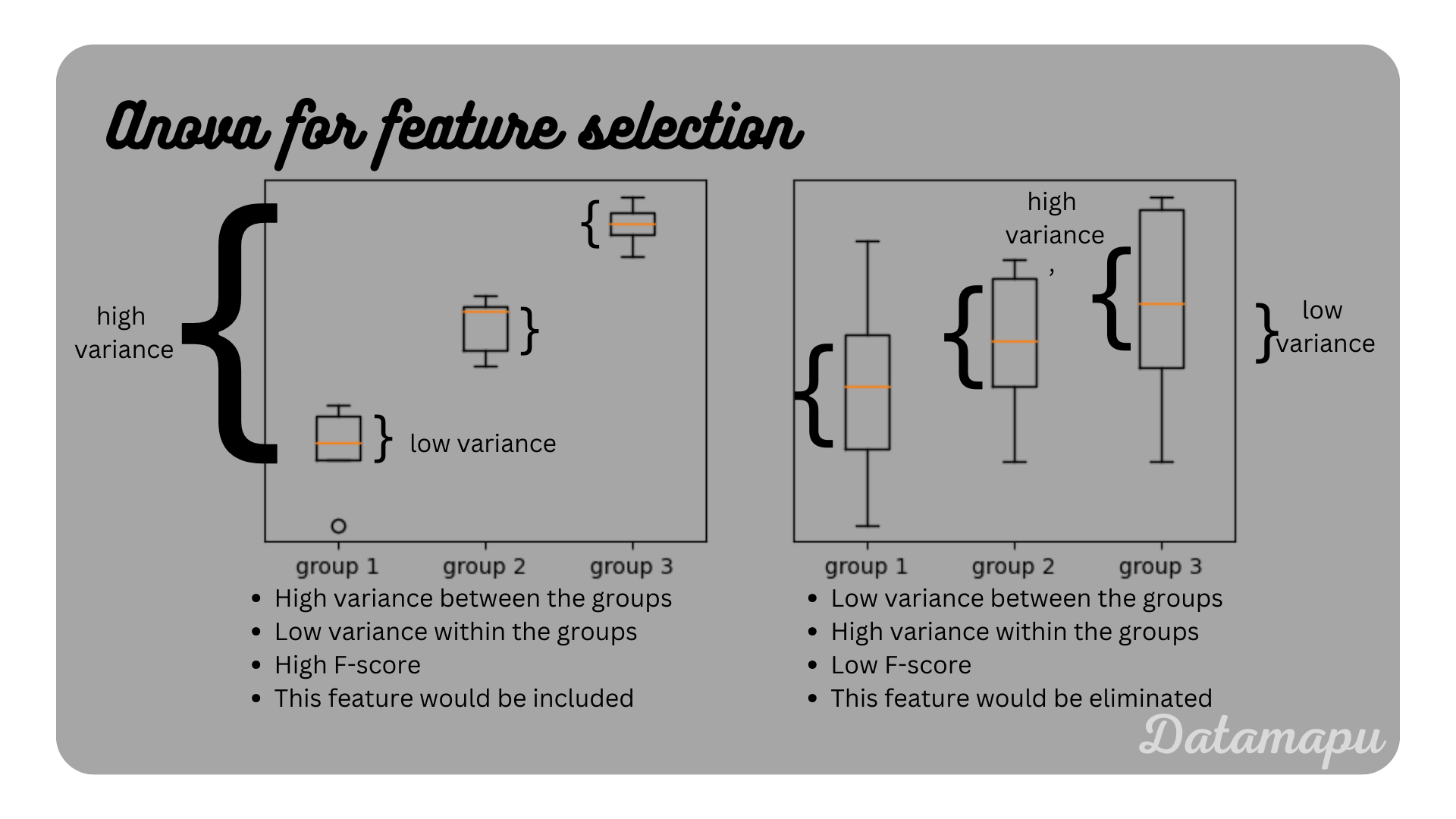
Analysis of Variance (ANOVA). ANOVA can be used when the target data is categorical. It aims to maximize the variance between the different classes, while minimizing the variance within each class. In other words, it determines whether the means of two or more groups for a particular feature differ significantly. For each feature the so-called F-Score is calculated, which is defined as the fraction of the variance between the groups divided by the variance within the groups. A feature is considered as important if the F-score is high. If a feature has a low variance between the classes, but a high variance within each class it is not considered as important, because it cannot be used to separate the classes. Two examples of a high F-score and a low F-score are illustrated in the plot below.

anova Illustration of variance within and between group variance in ANOVA.

Chi Square. The Chi-square test can be used to detect if an input feature has a strong relationship to the target data. It is used for classification problems when both input and target features are categorical. The Chi-square score is calculated for each feature and the target variable. The Chi-square score compares the observed and the expected counts of a category. A high score indicates a dependency between the feature and the target variable. The features with the highest scores are selected for training.

Embedded Methods

Embedded methods use a machine learning algorithm to select the most important features. The name results from the fact that the feature selection method is embedded into the machine learning algorithm itself. However, this algorithm may also be separated from the model used for training and only used for feature selection. We could fit one of the mentioned algorithms to our data, select the important features, and then use them in a different model. This algorithm is just fitted once, i.e. in contrast to wrapper methods, no retraining is needed. On the other hand, as in the wrapper methods interaction between the features is incorparated. They thus provide the advantages of both methods. Two examples are

Lasso Regulation. Lasso (L1) regulation is usually used to avoid overfitting by adding a penalty to the loss. A linear model can be used together with a L1 regulation to remove features that are not relevant. In a linear model the penalty is applied to the coefficients and L1 regularisation can set the coefficients of non-relevant features to zero. These features can then be removed.
Random Forest. Random Forests are built as a combination of several Decision Trees. A Decision Tree is constructed by separating the data in each node such that the impurity of the following node is maximally reduced. There are different ways to measure the impurity, especially depending on whether a classification or a regression is considered. The more the impurity is decreased the more important is this feature. The most important features are thus selected at the top of the tree and the less important features are more at the bottom. By pruning the tree, i.e. setting a maximal depth we can consider the features below that depth as not important. In a Random Forest, the decrease in impurity of each feature is then averaged over all trees.

Overview about the discussed methods for feature selection.

Summary

There are three different types of feature selection methods: wrapper methods, filter methods, and embedded methods. This post explains the most common ones, but of course, there are many more. Wrapper methods can evaluate a group of features together and analyze their interaction, while filter methods consider each feature individually. They usually result in a higher model performance than filter methods. However, wrapper methods are computationally more expensive and the feature selection is optimized for a specific model. Using a different model the results may change. Embedded methods use a dedicated machine learning model for the feature selection process and they combine both advantages of the other methods, i.e. they consider feature interactions and they are computationally lightweight.

If this blog is useful for you, please consider supporting.