AdaBoost - Explained
- 10 minutes read - 2030 wordsIntroduction
AdaBoost is an example of an ensemble supervised Machine Learning model. It consists of a sequential series of models, each one focussing on the errors of the previous one, trying to improve them. The most common underlying model is the Decision Tree, other models are however possible. In this post, we will introduce the algorithm of AdaBoost and have a look at a simplified example for a classification task using sklearn. For a more detailed exploration of this example - deriving it by hand - please refer to AdaBoost for Classification - Example. A more realistic example with a larger dataset is provided on kaggle. Accordingly, if you are interested in how AdaBoost is developed for a regression task, please check the article AdaBoost for Regression - Example.
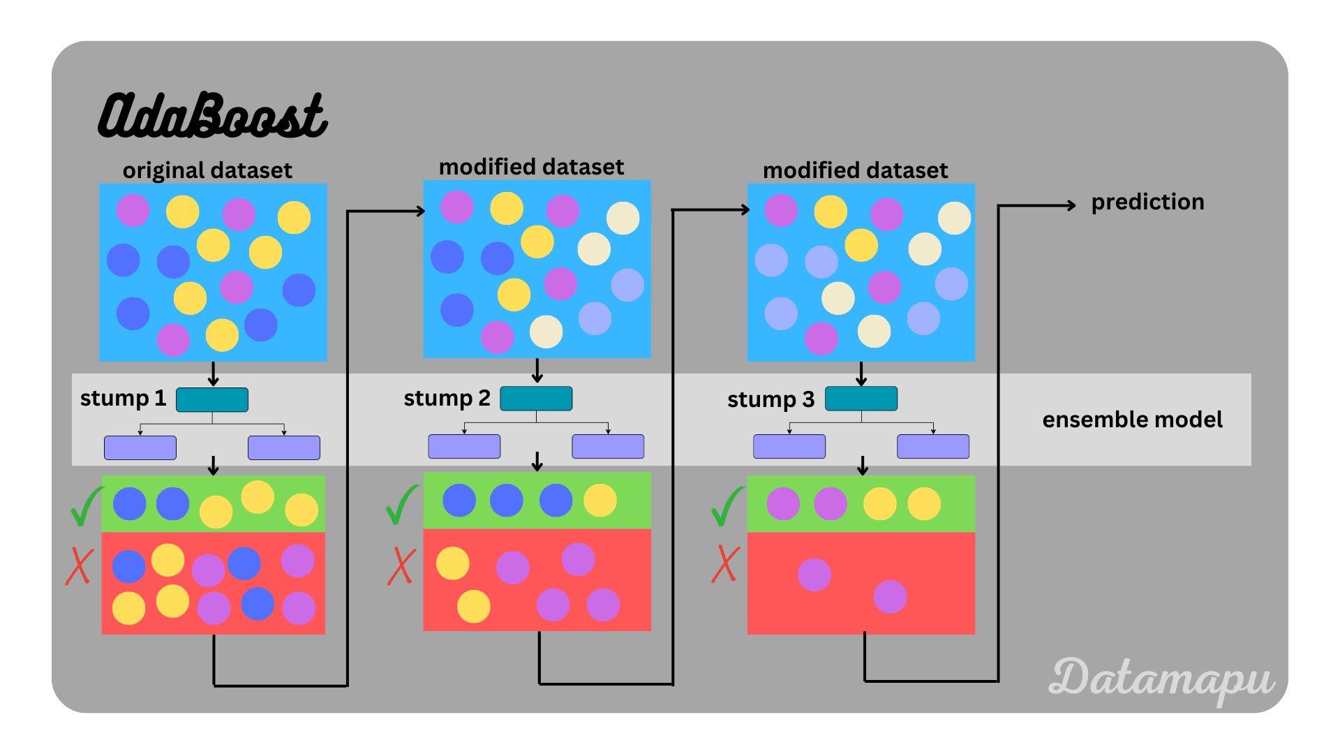 AdaBoost illustrated.
The Algorithm
The name AdaBoost is short for Adaptive Boosting, which already explains the main ideas of the algorithm. AdaBoost is a Boosting algorithm, which means that the ensemble model is built sequentially and each new model builds on the results of the previous one, trying to improve its errors. The developed models are all weak-learners, that is they have low predictive skill which is only slightly higher than random guessing. The word adaptive refers to the adaption of the weights that are assigned to each sample before fitting the next model. The weights are determined in such a way that the wrongly predicted samples get higher weights than the correctly predicted samples. In more detail, the algorithm works as follows.
- Fit a model to the initial dataset with equal weights. The first step is to assign a weight to each sample of the dataset. The initial weight is $\frac{1}{N}$, with $N$ being the number of data points. The weights always sum up to $1.$ Because in the beginning, all weights are equal, this means they can be ignored in this first step. If the base model is a Decision Tree, the weak learner is a very shallow tree or even only the stump, which refers to the tree that consists only of the root node and the first two leaves. How deep the tree is developed is a hyperparameter, that needs to be set. If we fit an AdaBoost algorithm in Python and use sklearn the default setting depends on whether a classification or a regression is considered. For classification, the default setting is to use stumps and for regression, the default value is a maximal depth of $3$.
- Make predictions and calculate the influence ($\alpha$) of the fitted model. Not only does the dataset get weights assigned, but also each model. We call the weights that are associated with each model their influence. The influence of a model on the final prediction depends on its error and is calculated as $$\alpha = \frac{1}{2} \ln\Big(\frac{1 - TotalError}{TotalError}\Big).$$ The Total Error is the sum of the sample weights for all wrongly predicted data points, which is always between $0$ and $1$. With $0$ meaning the model predicts all samples wrongly and $1$ meaning all samples are correctly predicted. How the influence $\alpha$ evolves depending on the Total Error is illustrated below. For values lower than $0.5,$ the model gets a negative influence, for values higher than $0.5$ it gets a positive influence, for exactly $0.5$ the influence is $0$.
- Adjust the weights of the data samples. The new weight ($w_{new}$) for each data sample is calculated as $$w_{new} = w_{old} * e^{\pm\alpha},$$ with $w_{old}$ the old or previous weight of that sample and $\alpha$ the influence of the model calculated in the previous step. The sign in the exponent changes depending on whether the sample was correctly predicted or not. If it was correctly predicted, the sign is negative, so that the weight decreases. On the other hand, if it was wrongly predicted, the sign is positive, so that the weight increases. Because the sum of all weights must be $1$, they are normalized, by dividing them by their sum.
- Create a weighted dataset. The calculated weights are now used to create a new dataset. For that, the calculated weights are used as bins for each sample. Let’s assume we calculated the weights $w_1, w_2, \dots, w_N$, the bin for the first sample is $0$ to $w_1$, the bin for the second sample is $w_1$ to $w_1+w_2$ and so on. Data samples are now selected by choosing $N$ random numbers between $0$ and $1$, with $N$ the number of data samples. For each of these random numbers, the sample is chosen in which bin the random number falls. Since wrongly predicted samples have higher weight than correctly predicted samples, their bins are larger. Therefore the probability of drawing a wrongly predicted sample is higher. The newly created dataset consists again of $N$ samples, but there are likely duplicates from the wrongly predicted samples.
- Fit a model to the new dataset. Now we start again and fit a model, equally to the first step, but this time using the modified dataset.
Repeat steps 2 to 5 $d$ times, where $d$ is the number of final weak learners of which the ensemble model is composed. It is a hyperparameter that needs to be chosen. You can find an example of these steps with detailed calculations in the articles AdaBoost for Classification - Example or AdaBoost for Regression - Example. For the final prediction of the ensemble model, predictions of all individual models are made. In a classification task, the influences of the different predictions are added and the majority is the final prediction. In a regression task, the weighted mean of the individual model prediction gives the final prediction, where the weights are the influences of the models.
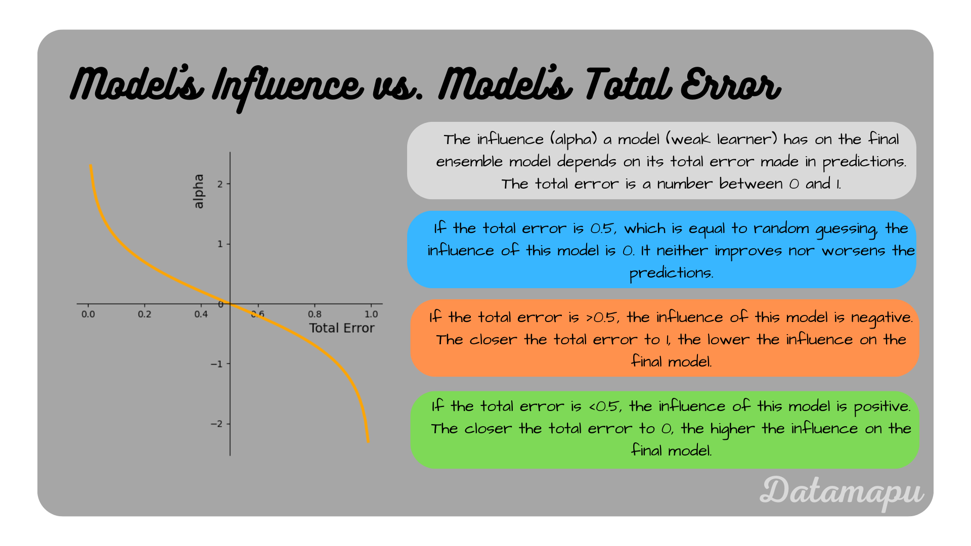 The influence of an individual model to the final ensemble model, depending on its total error.
AdaBoost vs. Random Forest
As mentioned earlier the most common way of constructing AdaBoost is using Decision Trees as underlying models. Another important ensemble machine learning model based on Decision Trees is the Random Forest. While Decision Trees are powerful machine learning algorithms, one of their major disadvantages is that they tend to overfit. Both, Random Forest and AdaBoost try to improve this while maintaining the advantages of Decision Trees, such as their robustness towards outliers and missing values. Both algorithms, however, differ substantially. In Adaboost, the weak learners associated are very short trees or even only the root node and the first two leaves, which is called the tree stump, whereas, in a Random Forest, all trees are built until the end. Stumps and very shallow trees are not using the entire information available from the data and are therefore not as good in making correct decisions. Another difference is, that in a Random Forest, all included Decision Trees are built independently, while in AdaBoost they build upon each other and each new tree tries to reduce the errors of the previous one. In other words, a Random Forest is an ensemble model based on Bagging, while AdaBoost is based on Boosting. Finally, in a Random Forest all trees are equally important, while in AdaBoost, the individual shallow trees / stumps have different influences because they are weighted differently. The following table summarizes the differences between Random Forests and AdaBoost based on Decision Trees.
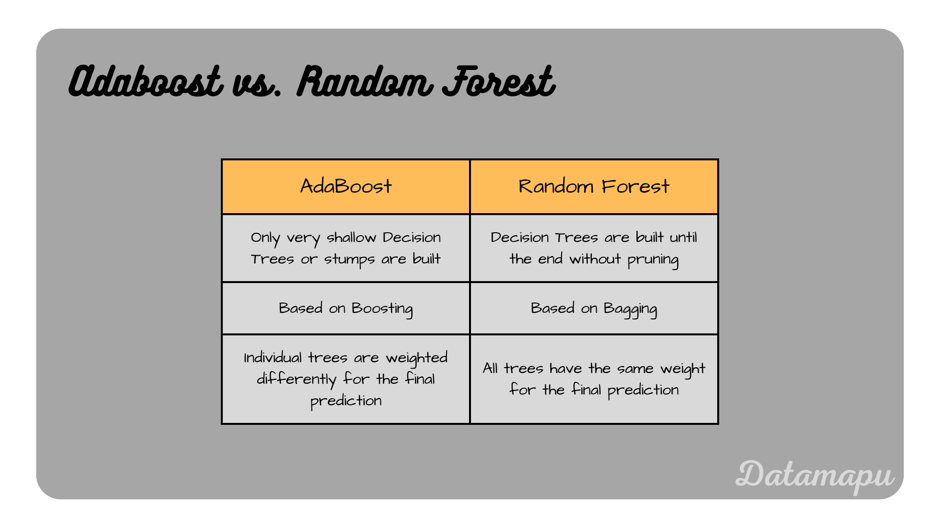 Main differences between AdaBoost and a Random Forest.
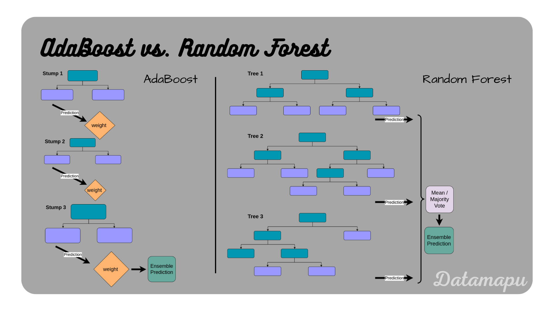 AdaBoost and Random Forest illustrated.
AdaBoost in Python
The sklearn library offers a method to fit AdaBoost in Python for both classification and regression problems. We will consider a simplified example for a classification task, using the following data, which describes whether a person should go rock climbing or not depending on their age and whether they like height and goats.
| |
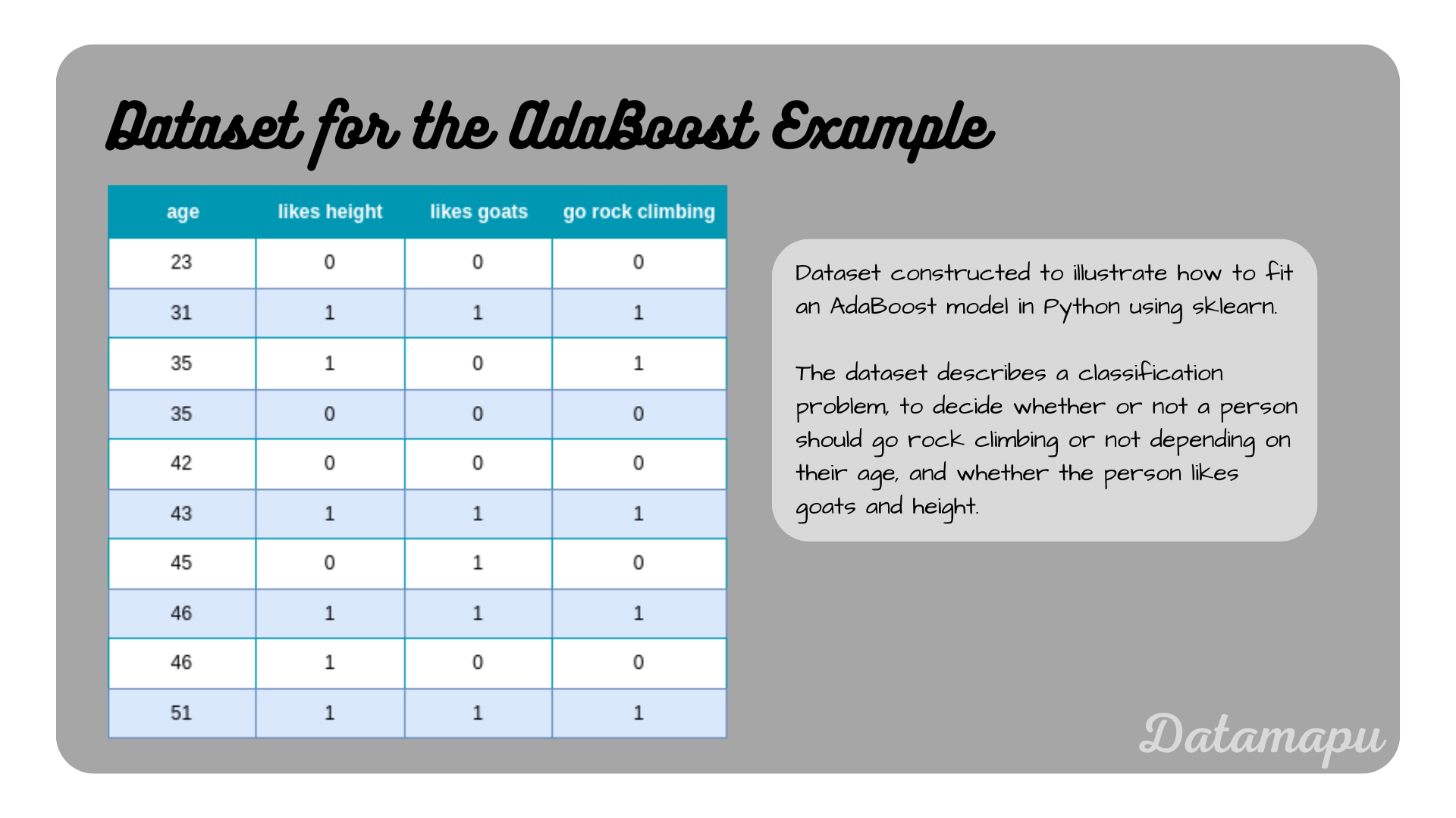 Example dataset to illustrate AdaBoost in Python.
We use this data to fit an AdaBoost Classifier. As this is a very simplified dataset, we use only three models to build the ensemble model. This is done by setting the hyperparameter n_estimators=3. The other hyperparameters are left as the default values. That means as base models the stumps of Decision Trees are used.
| |
To make predictions we can use the predict method, and then we can print the score, which is defined as the mean accuracy.
| |
The predictions are $[0, 1, 1, 0, 0, 1, 0, 1, 0, 1]$ and the score is $1.0$. That means our model predicts all samples correctly. We can also print the predictions and scores for each boosting iteration, to see how the individual models perform.
| |
The predictions for the three stages are
stage 1: $[0, 1, 1, 0, 0, 1, 0, 1, 1, 1]$,
stage 2: $[0, 1, 0, 0, 0, 1, 0, 1, 0, 1]$, and
stage 3 $[0, 1, 1, 0, 0, 1, 0, 1, 0, 1]$.
Accordingly the scores are
stage 1: $0.9$,
stage 2: $0.9$, and
stage 3: $1.0$.
The weights for the individual trees can be achieved by
| |
which for this example shows, that all three estimators have weight $1$. Note, that sklearn gives a weight of $1$, although the individual models show Total Errors greater than $0$. This is due to a different implementation of the algorithm. By the time, writing this post the default algorithm in sklearn is SAMME.R.. A discussion about why the weights are $1$ can be found on stackoverflow. The final prediction is then achieved by adding up the weights for each class predicted and the larger value is the final prediction. Since the weights in this case are all $1$, it is the same as the majority vote.
To illustrate the model we can plot the three stumps created. We can access them using the estimators_ attribute. Note that creating the stumps includes randomness when the modified dataset is constructed, as described above. To make the results reproducible the random_seed is set when fitting the model. The first tree stump can be visualized as follows.
| |
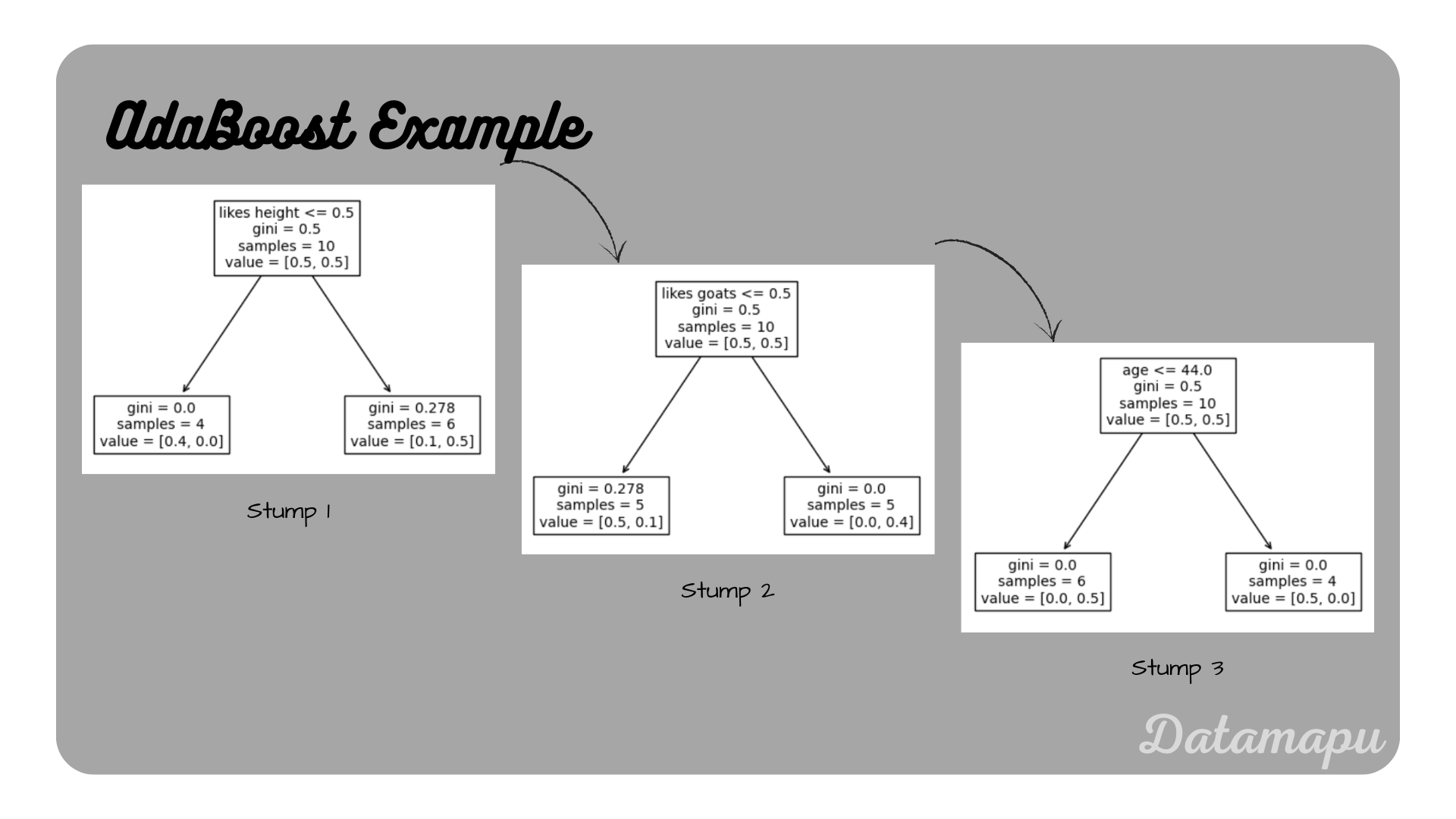 The three stumps for the AdaBoost model of the example.
Comparing the first stump to the calculations in the article Decision Trees for Classification - Example, in which the same dataset is used, we can see that this is exactly the beginning of the Decision Tree developed. Please find a detailed derivation of the above example, calculating it by hand in the separate article AdaBoost for Classification - Example. In a real project, we would of course divide our data into training, validation, and test data, and then fit the model to the training data only and evaluate on validation and finally on the test data. A more realistic example is provided on kaggle
Summary
AdaBoost is an ensemble model, in which a sequential series of models is developed. Sequentially the errors of the developed models are evaluated and the dataset is modified such that a higher focus lies on the wrongly predicted samples for the next iteration. In Python, we can use sklearn to fit an AdaBoost model, which also offers some methods to explore the created models and their predictions. It is important to note, that different implementations of this algorithm exist. Due to this and the randomness in the bootstrapping, there are some differences, when we compare the details to the model fitted using sklearn. The example used in this article was very simplified and only for illustration purposes. For a more developed example in Python, please refer to kaggle.
If this blog is useful for you, please consider supporting.
