Gradient Boost for Classification Example

April 28, 2024 - 8 minutes read - 1548 words

Introduction

In this post, we develop a Gradient Boosting model for a binary classification. We focus on the calculations of each single step for a specific example chosen. For a more general explanation of the algorithm and the derivation of the formulas for the individual steps, please refer to Gradient Boost for Classification - Explained and Gradient Boost for Regression - Explained. Additionally, we show a simple example of how to apply Gradient Boosting for classification in Python.

Data

The dataset used for this example contains 10 samples and describes the task of whether a person should go rock climbing depending on their age, and whether the person likes height and goats. The same dataset was used in the articles Decision Trees for Classification - Example, and Adaboost for Classification - Example.

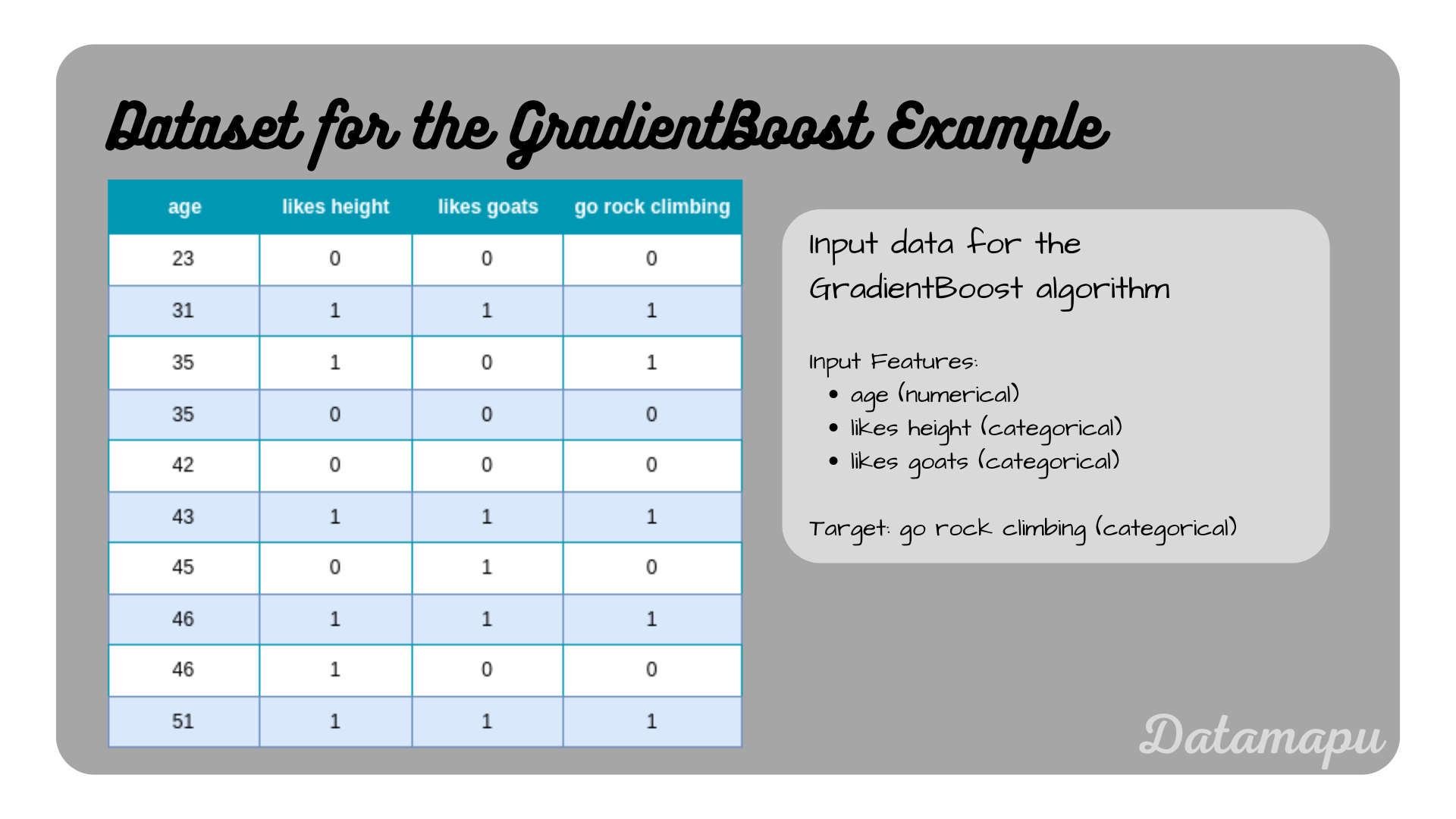“data” The data used in this post.

Build the Model

We build a Gradient Boosting model using pruned Decision Trees as weak learners for the above dataset. The steps to be performed are summarized in the plot below. For a more detailed explanation please refer to Gradient Boost for Classification - Explained.

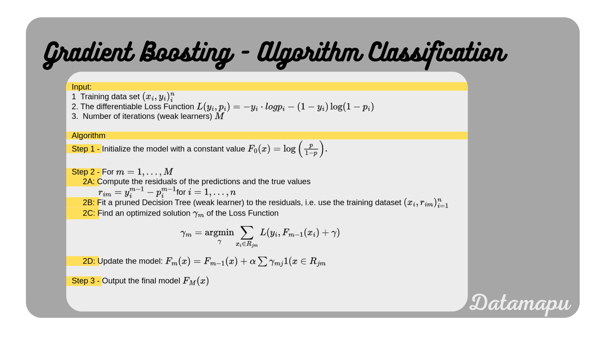Gradient Boosting for Classification Gradient Boosting Algorithm simplified for a binary classification task.

Step 1 - Initialize the model with a constant value - $F_{0} (X) = \log (\frac{p}{1 - p})$ .

For the first initialization, we need the probability of “go rock climbing”. In the above dataset, we have five $1$ s and five $0$ s, and a total dataset size of ten samples. That is the probability of “going rock climbing” is $\frac{5}{10} = 0.5$ . With that, we can calculate

$F_{0} (X) = \log (\frac{P (y = 1)}{P (y = 0)}) = \log (\frac{0.5}{0.5}) = 0.$

The initial log-loss in this case is $0$ , which means that the chances of both outcomes of the target variable are equal. The initial predictions are thus $F_{0} (X) = [0, 0, 0, 0, 0, 0, 0, 0, 0, 0]$

To check the performance of our model, we use the accuracy score. We calculate the accuracy after each step, to see how the model evolves. For the initial predictions, we first calculate the probabilities.

$p_{0} = \frac{1}{1 + e^{- F_{0} (X)}} = [0.5, 0.5, 0.5, 0.5, 0.5, 0.5, 0.5, 0.5, 0.5, 0.5]$

As a threshold for predicting a $1$ we use $0.5$ . In this case, the predictions are

${\hat{y}}_{0} = [1, 1, 1, 1, 1, 1, 1, 1, 1, 1]$ .

The accuracy is calculated as the fraction of the correct predicted values and the total number of samples

$a c c u r a c y = \frac{5}{10} = 0.5$

Step 2 - For $m = 1$ to $M = 2$ :

In this step we sequentially fit weak learners (pruned Decision Trees) to the residuals. The number of loops is the number of weak learners considered. Because the data considered in this post is so simple, we will only loop twice, i.e. .

First loop $M = 1$

Fit the first Decision Tree.

2A. Compute the residuals of the preditions and the true observations.

The residuals are calculated as

$r_{1} = y - p_{0} = [- 0.5, 0.5, 0.5, - 0.5, - 0.5, 0.5, - 0.5, 0.5, - 0.5, 0.5]$

2B. and 2C. Fit a model (weak learner) to the residuals and find the optimized solution.

In this step, we use the above calculated residuals to fit a Decision Tree. We prune the tree to use it as a weak learner. We use a maximum depth of two. We don’t develop the Decision Tree by hand, but will use the sklearn method DecisionTreeClassifier. For a step-by-step example of building a Decision Tree for Classification, please refer to the article Decision Trees for Classification - Example.

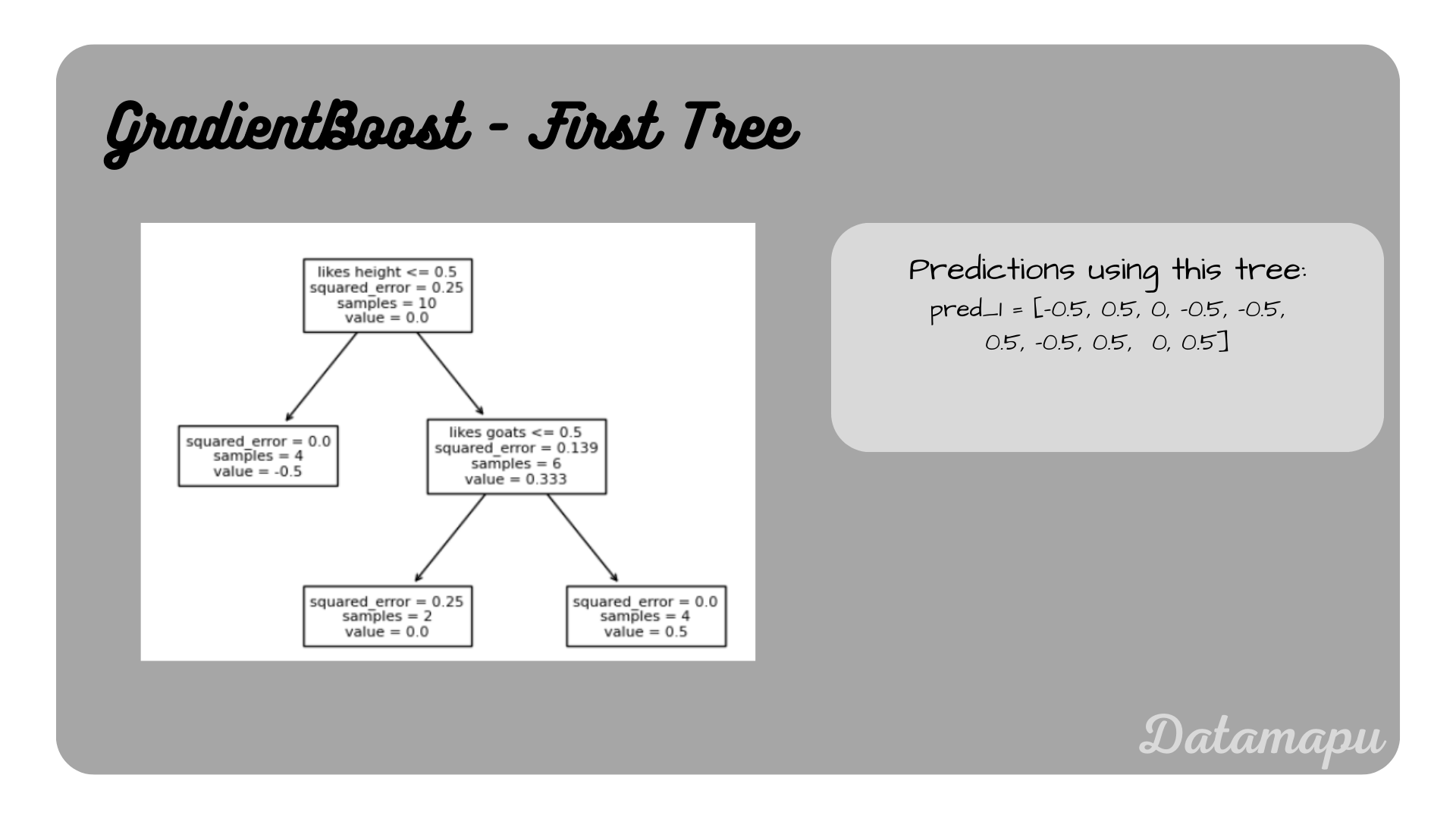“first tree” First Decision Tree, i.e. first weak learner

The resulting predictions are

$p r e d_{1} (X) = [- 0.5, 0.5, 0., - 0.5, - 0.5, 0.5, - 0.5, 0.5, 0., 0.5]$

2D. Update the model.

We update the model using the predictions of the above developed Decision Tree. We use a learning rate of $α = 0.3$ for this example. This results in the updated model

$F_{1} (X) = F_{0} (X) + 0.3 * p r e d_{1} (X) .$

Using the calculated numbers, this leads to

$F_{1} (X) = [0, 0, 0, 0, 0, 0, 0, 0, 0, 0] + 0.3 \cdot [- 0.5, 0.5, 0., - 0.5, - 0.5, 0.5, - 0.5, 0.5, 0., 0.5]$ $F_{1} (X) = [- 0.15, 0.15, 0, - 0.15, - 0.15, 0.15, - 0.15, 0.15, 0, 0.15]$

The probabilies resulting from these log-loss are

$p_{1} = \frac{1}{1 + e^{- F_{1} (X)}} = [0.46, 0.54, 0.5, 0.46, 0.46, 0.54, 0.46, 0.54, 0.5, 0.54] .$

With the threshold of $0.5$ this leads to the predictions

${\hat{y}}_{2} (X) = [0, 1, 1, 0, 0, 1, 0, 1, 1, 1] .$

The accuracy after this step is

$a c c u r a c y = \frac{9}{10} = 0.9 .$

Second loop $M = 2$

Fit the second Decision Tree.

2A. Compute the residuals of the preditions and the true observations

The residuals are calculated as

$r_{2} = y - p_{1} = [- 0.46, 0.46, 0.5, - 0.46, - 0.46, 0.46, - 0.46, 0.46, - 0.5, 0.46]$

2B. and 2C. Fit a model (weak learner) to the residuals and find the optimized solution.

Now we fit the second Decision Tree with the residuals $r_{2}$ calculated above as target.

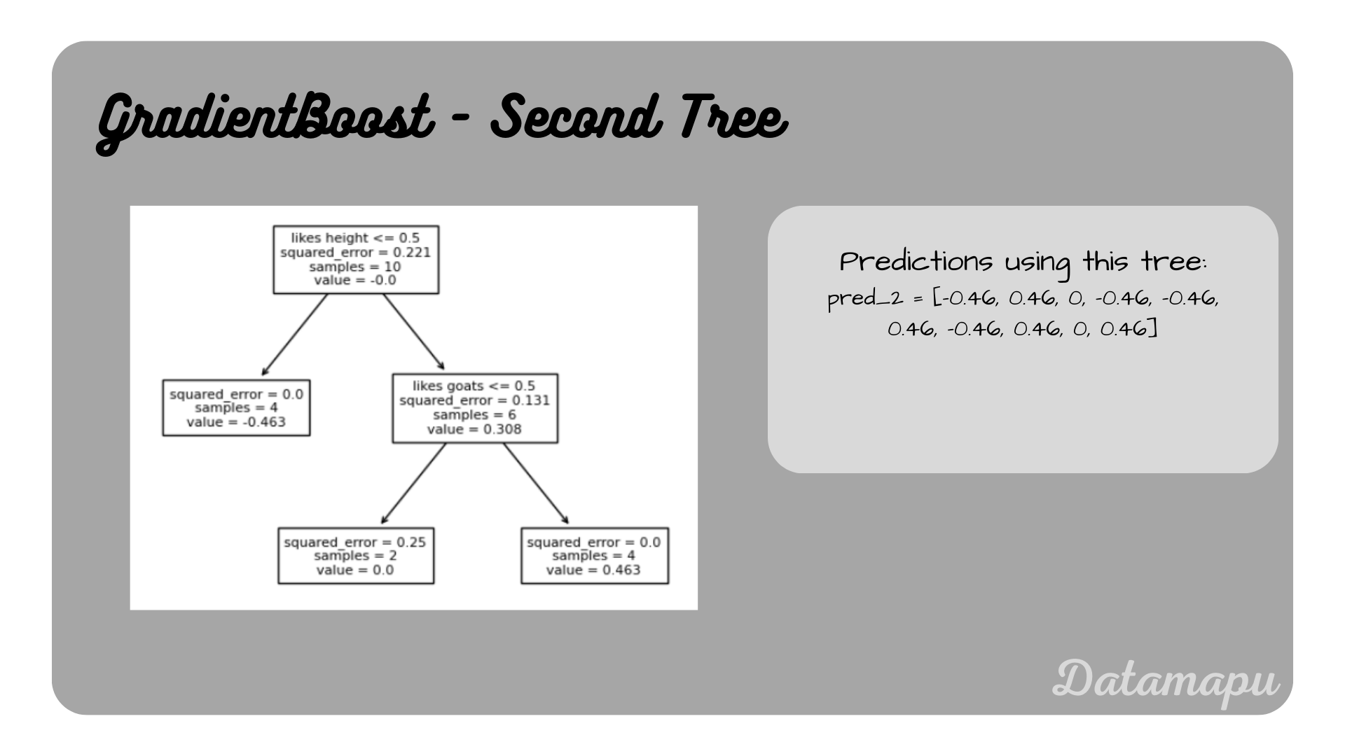“second tree” Second Decision Tree, i.e. second weak learner

The resulting predictions are

$p r e d_{2} (X) = [- 0.46, 0.46, 0, - 0.46, - 0.46, 0.46, - 0.46, 0.46, 0, 0.46]$

2D. Update the model.

We again update the model using the predictions of this second Decision Tree with a learning rate of $0.3$ . This results in the updated model

$F_{2} (X) = F_{1} (X) + 0.3 \cdot p r e d_{2} (X) .$

Using the calculated numbers, this leads to

$F_{2} (X) = [- 0.15, 0.15, 0, - 0.15, - 0.15, 0.15, - 0.15, 0.15, 0, 0.15] +$ $0.3 \cdot [- 0.46, 0.46, 0, - 0.46, - 0.46, 0.46, - 0.46, 0.46, 0, 0.46]$ $F_{2} (X) = [- 0.29, 0.29, 0, - 0.29, - 0.29, 0.29, - 0.29, 0.29, 0, 0.29]$

The probabilies resulting from these log-loss are

$p_{2} = \frac{1}{1 + e^{- F_{2} (X)}} = [0.43, 0.57, 0.5, 0.43, 0.43, 0.57, 0.43, 0.57, 0.5, 0.57] .$

With the threshold of $0.5$ this leads to the predictions

${\hat{y}}_{3} = [0, 1, 1, 0, 0, 1, 0, 1, 1, 1] .$

The accuracy after this step is

$a c c u r a c y = \frac{9}{10} = 0.9 .$

That is, this second step didn’t improve the accuracy of our model.

Step 3 - Output final model $F_{M} (x)$ .

The final model then in defined by the output of the last step

$F_{2} (X) = F_{0} (X) + α \cdot F_{1} (X) + α \cdot p r e d_{2} .$

Using the input features $X$ given in the above table, this is

$F_{2} (X) = [- 0.29, 0.29, 0, - 0.29, - 0.29, 0.29, - 0.29, 0.29, 0, 0.29] .$

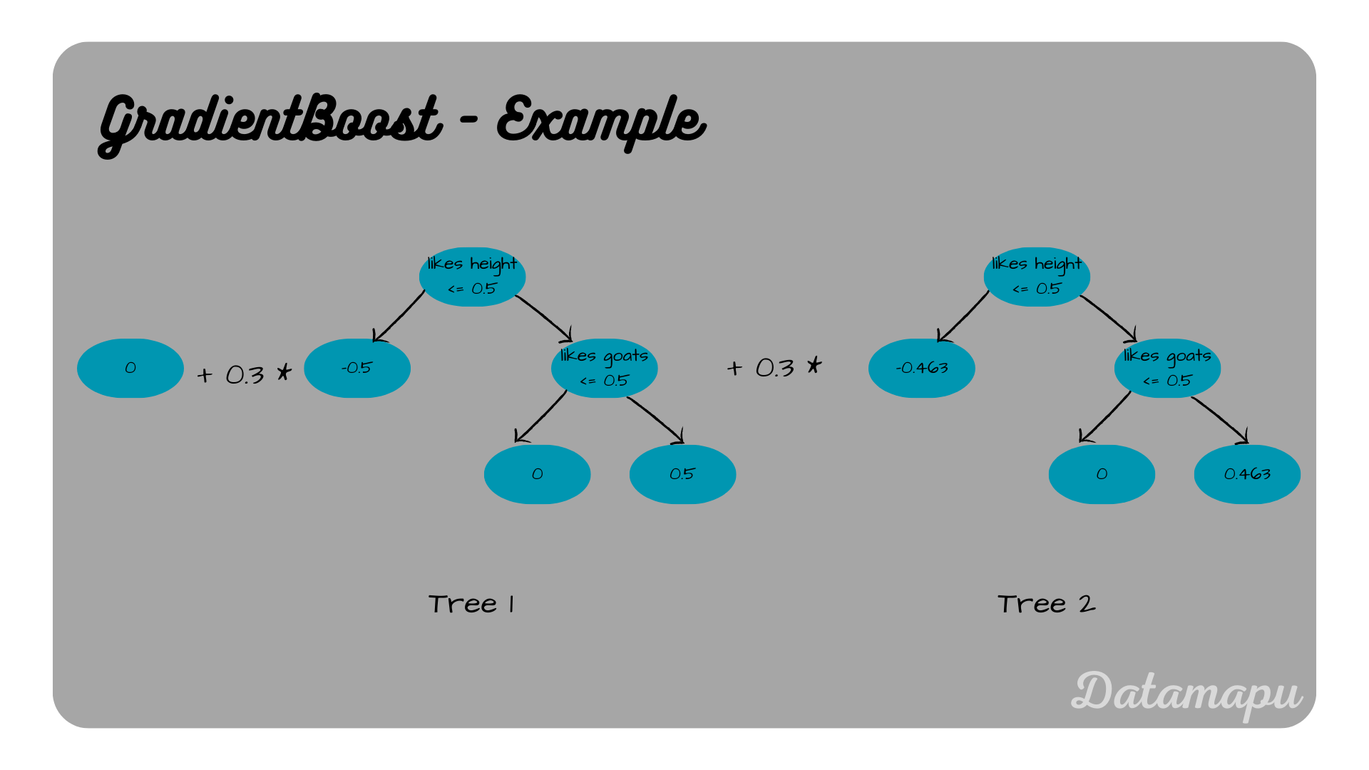“final model” Final model.

Accordingly the final probabilities $p_{2}$ and predictions ${\hat{y}}_{3}$ as calculated in the last step of the above loop.

Fit a Model in Python

In this section, we will show how to fit a GradientBoostingClassifier from the sklearn library to the above data. In sklearn the weak learners are fixed to Decision Trees and cannot be changed. The GradientBoostingClassifier offers a set of hyperparameters, that can be changed and tested to improve the model. Note, that we are considering a very simplified example. In this case, we set the number of weak learners (n_estimators) to $2$ , the maximal depth (max_depth) of the Decision Trees to $2$ , and the learning_rate= $0.3$ . For real-world data, usually, hyperparameters are chosen differently, the default values in sklearn are n_estimators $= 100$ , max_depth $= 3$ , and the learning_rate= $0.1$ . For a complete list of available hyperparameters, please refer to the sklearn documentation.

We read the data into a Pandas dataframe.

1
2
3
4
5
6
7
8
import pandas as pd

data = {'age': [23, 31, 35, 35, 42, 43, 45, 46, 46, 51],
        'likes goats': [0, 1, 0, 0, 0, 1, 1, 1, 0, 1],
        'likes height': [0, 1, 1, 0, 0, 1, 0, 1, 1, 1],
        'go rock climbing': [0, 1, 1, 0, 0, 1, 0, 1, 0, 1]}

df = pd.DataFrame(data)

Now we can fit the model using the above defined hyperparameters.

 1
 2
 3
 4
 5
 6
 7
 8
 9
10
from sklearn.ensemble import GradientBoostingClassifier

X = df[['age', 'likes goats', 'likes height']].values
y = df[['go rock climbing']].values.reshape(-1,)
clf = GradientBoostingClassifier(
    n_estimators=2,
    max_depth=2,
    learning_rate=0.3	
    )
clf.fit(X, y)

The GradientBoostingClassifier has a predict method, which we can use to get the predictions and the score method to calculate the accuracy.

1
2
y_pred = clf.predict(X)
score = clf.score(X, y)

We get the predictions $[0, 1, 0, 0, 0, 1, 0, 1, 0, 1]$ and a score of $0.9$ . A more detailed example of applying Gradient Boosting in Python can be found on kaggle - this is an example of a regression problem. The application to a classification problem, however, is the same, we only need to change the GradientBoostingRegressor to the GradientBoostingClassifier and change the metrics to evaluate the model.

Summary

In this post, we went through the calculations of the individual steps to build a Gradient Boosting model for a binary classification problem. A simple example was chosen to make explicit calculations feasible. Later, we showed how to fit a model using Python. In real-world examples, libraries like sklearn are used to develop such models. The development is usually not as straightforward as in this simplified example, but a set of hyperparameters are (systematically) tested to optimize the solution. For a more detailed explanation of the algorithm, please refer to the related articles Gradient Boost for Classification - Explained, Gradient Boost for Regression - Explained, Gradient Boost for Regression - Example. For a more practical approach, please check the notebook on kaggle, where a Gradient Boosting model for a regression problem is developed.

If this blog is useful for you, please consider supporting.

Introduction

Data

Build the Model

Step 1 - Initialize the model with a constant value - F0(X)=log⁡(p1−p).

Step 2 - For m=1 to M=2:

First loop M=1

2A. Compute the residuals of the preditions and the true observations.

2B. and 2C. Fit a model (weak learner) to the residuals and find the optimized solution.

2D. Update the model.

Second loop M=2

2A. Compute the residuals of the preditions and the true observations

2B. and 2C. Fit a model (weak learner) to the residuals and find the optimized solution.

2D. Update the model.

Step 3 - Output final model FM(x).

Fit a Model in Python

Summary

Step 1 - Initialize the model with a constant value - $F_{0} (X) = \log (\frac{p}{1 - p})$ .

Step 2 - For $m = 1$ to $M = 2$ :

First loop $M = 1$

Second loop $M = 2$

Step 3 - Output final model $F_{M} (x)$ .