Gradient Boost for Regression - Example

April 9, 2024 - 8 minutes read - 1581 words

Introduction

In this post, we will go through the development of a Gradient Boosting model for a regression problem, considering a simplified example. We calculate the individual steps in detail, which are defined and explained in the separate post Gradient Boost for Regression - Explained. Please refer to this post for a more general and detailed explanation of the algorithm.

Data

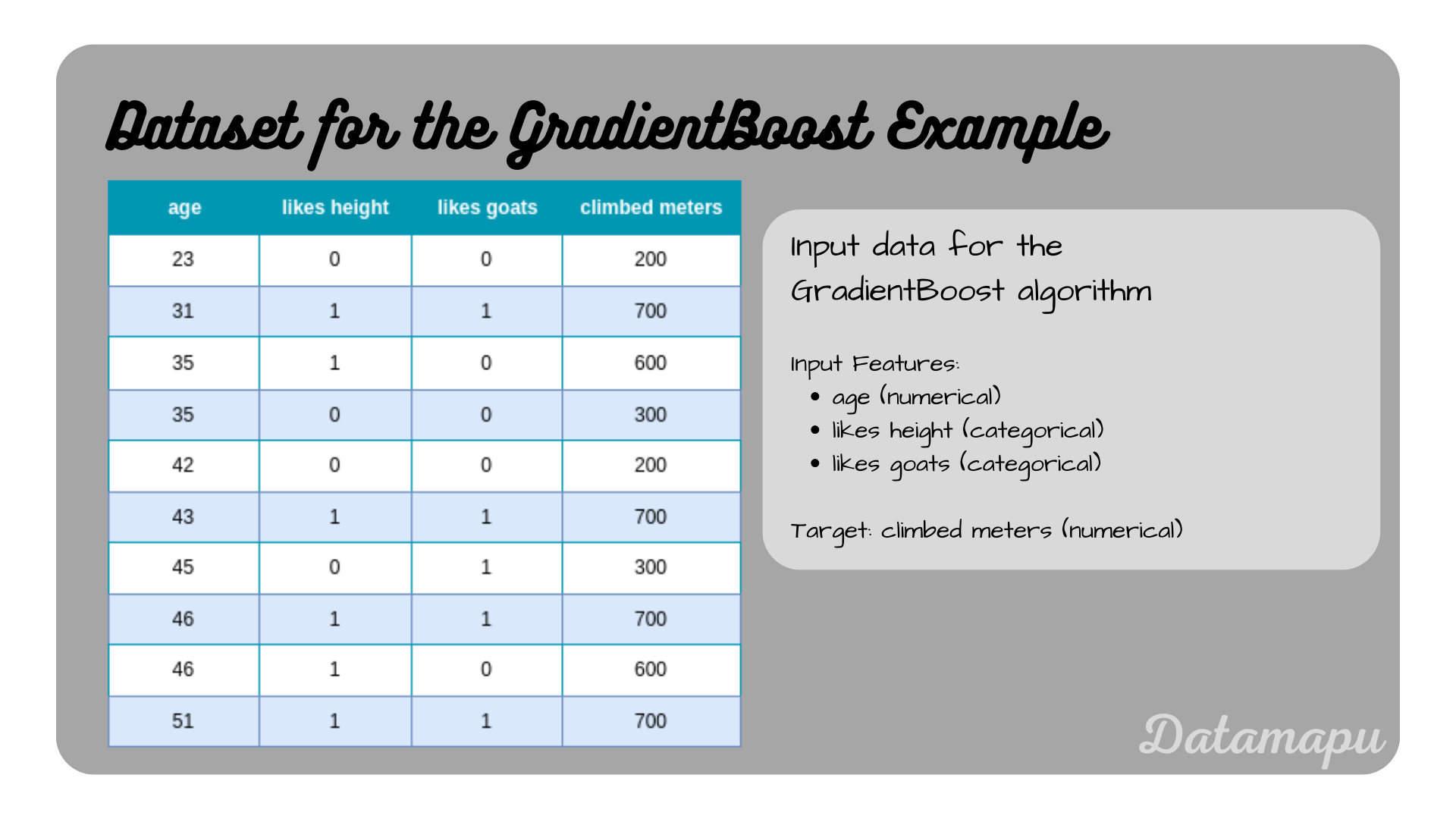
We will use a simplified dataset consisting of only 10 samples, which describes how many meters a person has climbed, depending on their age, whether they like height, and whether they like goats. We used that same data in previous posts, such as Decision Trees for Regression - Example, and Adaboost for Regression - Example.

“data” The data used in this post.

Build the Model

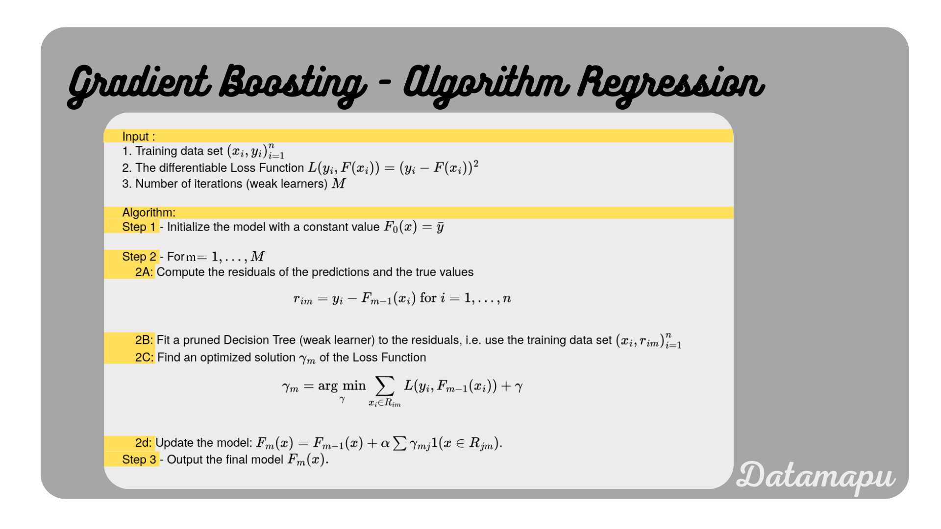
We build a Gradient Boost model with pruned Decision Trees as weak learners using the above dataset. For that, we follow the steps summarized in the following plot. For a more detailed explanation please refer to Gradient Boost for Regression - Explained.

Gradient Boosting for Regression Gradient Boosting Algorithm simplified for a regression task.

Step 1 - Initialize the model with a constant value - $F_0(X) = \bar{y}$.

The initialization of the model is done by taking the means of all target values ($y = $ “climbed meters”). In our case

$$F_0(X) = \frac{1}{10}(200 + 700 + 600 + 300 + 200 + 700 + 300 + 700 + 600 + 700) = 500.$$

To evaluate how the model evolves, we calculate the mean squared error (MSE) after each iteration.

$$MSE(y, F_0(X)) = \frac{1}{10}((200 - 500)^2 + (700 - 500)^2 + (600 - 500)^2 + $$ $$(300 - 500)^2 + (200 - 500)^2 + (700 - 500)^2 + (300 - 500)^2 + $$ $$(700 - 500)^2 + (600 - 500)^2 + (700 - 500)^2) = 44 000$$

The MSE of this first estimate is $44 000$ m.

Step 2 - For $m=1$ to $M=2$:

The second step is a loop, which sequentially updates the model by fitting a weak learner, in our case a pruned Decision Tree to the residual of the target values and the previous predictions. The number of loops is the number of weak learners considered. Because the data considered in this post is so simple, we will only loop twice, i.e. $M=2$.

First loop $M=1$

2A. Compute the residuals of the preditions and the true observations.

With $X$ the input features “age”, “likes height”, and “likes oats”, given in the previous table, we compute the residual as a vector

$$r_1 = y - F_0(X) = [(200 - 500), (700 - 500), (600 - 500), (300 - 500), $$ $$(200 - 500), (700 - 500), (300 - 500), (700 - 500), (600 - 500), (700 - 500)]$$

This results in

$$r_1 = [-300, 200, 100, -200, -300, 200, -200, 200, 100, 200].$$

2B. anc 2C. Fit a model (weak learner) to the residuals and find the optimized solution.

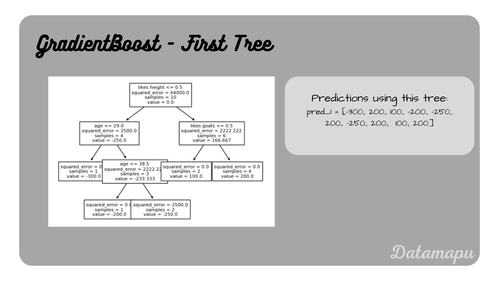
Now we fit a Decision Tree to the residuals ($r_1$) with the original target values. In this example, we set max_depth=3 in the Decision Tree to prune it. We will not develop the Decision Tree in detail but will use the result from sklearn. To follow a step-by-step example of building a Decision Tree for Regression, please refer to the separate article Decision Trees for Regression - Example.

“first tree” First Decision Tree, i.e. first weak learner

2D. Update the model.

The next step is to update the model with the new prediction from the weak learner.

$$F_1(X) = F_0(x) + pred_1 = [(500 - 300), (500 + 200), (500 + 100), (500 + -200),$$ $$(500 -250), (500 + 200), (500 - 250), (500 - 200), (500 + 100), (500 + 200)]$$

This results in

$$F_1(X) = [200, 700, 600, 300, 250, 700, 250, 700, 600, 700].$$

The MSE of these new predictions are

$$MSE(y, F_1(X)) = \frac{1}{10}((200 - 200)^2 + (700 - 700)^2 + (600 - 600)^2 + $$ $$(300 - 300)^2 + (200 - 250)^2 + (700 - 700)^2 + (300 - 250)^2 + $$ $$(700 - 700)^2 + (600 - 600)^2 + (700 - 700)^2) = 500$$

We can see that the error after this first update reduced to $500$ m.

Second loop $M=2$

In this second loop the same steps as in the first one are performed.

2A. Compute the residuals of the preditions and the true observations.

We start with computing the residuals between the target values ($y$ = “climbed meters”) and the current prediction.

$$r_2 = y - F_1(X) = [(200 - 200), (700 - 700), (600 - 600), (300 - 300), $$ $$(200 - 250), (700 - 700), (300 - 250), (700 - 700), (600 - 600), (700 - 700)]$$

This results in

$$r_2 = [0, 0, 0, 0, -50, 0, -50, 0, 0, 0].$$

2B. and 2C. Fit a model (weak learner) to the residuals and find the optimized solution.

We fit a Decision Tree to the newly calculated residuals $r_2$ and the target values.

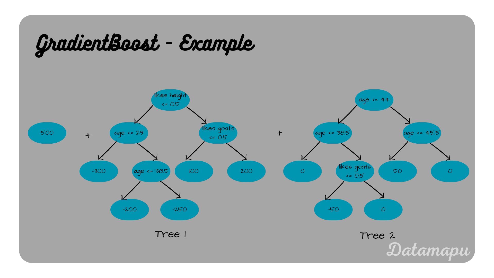
“second tree” Second Decision Tree, i.e. second weak learner

2D. Update the model.

The current model is updated using the predictions obtained from the above Decision Tree.

$$F_2(X) = F_1(X) + pred_2 = [(200 + 0), (700 + 0), (600 + 0), (300 + 0), $$ $$(250 - 50), (700 + 0), (250 + 50), (700 + 0), (600 + 0), (700 + 0)]$$

This results in

$$F_2(X) = [200, 700, 600, 300, 200, 700, 300, 700, 600, 700].$$

The MSE of this updated prediction is

$$MSE(y, F_2(X)) = \frac{1}{10}((200 - 200)^2 + (700 - 700)^2 + (600 - 600)^2 + $$ $$(300 - 300)^2 + (200 - 200)^2 + (700 - 700)^2 + (300 - 300)^2 + $$ $$(700 - 700)^2 + (600 - 600)^2 + (700 - 700)^2) = 0$$

That is we see another reduction in the error. Because of the simplicity of the data, in this case, the error is already $0$ m after two iterations. In real-world projects with more complex data, the number of weak learners is much higher. The default value in sklearn is $100$.

Step 3 - Output final model $F_M(x)$.

The result of this last step in the loop, then defines the final model.

$$F_2(X) = F_0(X) + F_1(X) + pred_2$$

For $x$ the input features given in the above table, this is

$$F_2(X) = [200, 700, 600, 300, 200, 700, 300, 700, 600, 700].$$

“final model” Final model.

Note, that usually an additional hyperparameter is used in Gradient Boosting, which is the learning rate. The learning rate determines the contribution of the trees. That is the predictions are scaled by the learning rate before adding them. In the above example, we thus used a learning rate of $1$, usually the learning rate is smaller, in sklearn the default value is $0.1$.

Including a learning rate $\alpha$ the formular for the final model is

$$F_n(X) = F_0(X) + \alpha \big(\sum_{i=1}^{n-1} F_i(X) + pred_n),$$

with $n$ the number of weak learners.

Fit a Model in Python

Python’s sklearn library provides a gradient boosting package. We can use this library to fit a simple model to our example data. You can find a more complex example with a more realistic dataset on kaggle.

Let’s read the data as a Pandas dataframe.

1
2
3
4
5
6
7
8
import pandas as pd

data = {'age': [23, 31, 35, 35, 42, 43, 45, 46, 46, 51],
        'likes goats': [0, 1, 0, 0, 0, 1, 1, 1, 0, 1],
        'likes height': [0, 1, 1, 0, 0, 1, 0, 1, 1, 1],
        'climbed meters': [200, 700, 600, 300, 200, 700, 300, 700, 600, 700]}

df = pd.DataFrame(data)

There are several hyperparameters that can be changed in the gradient boosting model of sklearn. A full list can be found in the sklearn documentation. In this example, we change the hyperparameters n_estimators, which defines the number of Decision Trees used as weak learners, max_depth, which defines the maximal depth of the Decision Trees, and the learning_rate, which defines the weight of each tree. The learning rate is a hyperparameter that we did not use in the algorithm above. The idea is similar as in the algorithm of Adaboost to give a weight to the weak learner. That is in the calculations above, this weight was set to $1$. With the hyperparameters as used in the above example, we fit the model as follows.

 1
 2
 3
 4
 5
 6
 7
 8
 9
10
11
from sklearn.ensemble import GradientBoostingRegressor

X = df[['age', 'likes goats', 'likes height']].values
y = df[['climbed meters']].values.reshape(-1,)
reg = GradientBoostingRegressor(
	n_estimators=2, 
	max_depth=3, 
	learning_rate=1, 
	random_state=42
	)
reg.fit(X, y)

Using the predict method gives us the predictions. We also calculate the score of the prediction. The score in this case is the Coefficient of Determination often abbreviated as $R^2$.

1
2
y_pred = reg.predict(X)
score = reg.score(X, y)

In this case this leads to a perfect predictions $[200, 700, 600, 300, 200, 700, 300, 700, 600, 700]$ and a score of $1$. A more detailed example using a larger dataset can be found on kaggle.

Summary

In this post, we calculated the individual steps for a Gradient Boosting model for a regression problem. We saw how updating the model by creating an ensemble model improves the results. This example was chosen on purpose for a very simple dataset in order to follow the calculations and understand each step. A more general description and explanation of the algorithm is given in the separate article Gradient Boost for Regression - Explained.

If this blog is useful for you, please consider supporting.