Backpropagation Step by Step

Introduction

A neural network consists of a set of parameters - the weights and biases - which define the outcome of the network, that is the predictions. When training a neural network we aim to adjust these weights and biases such that the predictions improve. To achieve that Backpropagation is used. In this post, we discuss how backpropagation works, and explain it in detail for three simple examples. The first two examples will contain all the calculations, for the last one we will only illustrate the equations that need to be calculated. We will not go into the general formulation of the backpropagation algorithm but will give some further readings at the end.

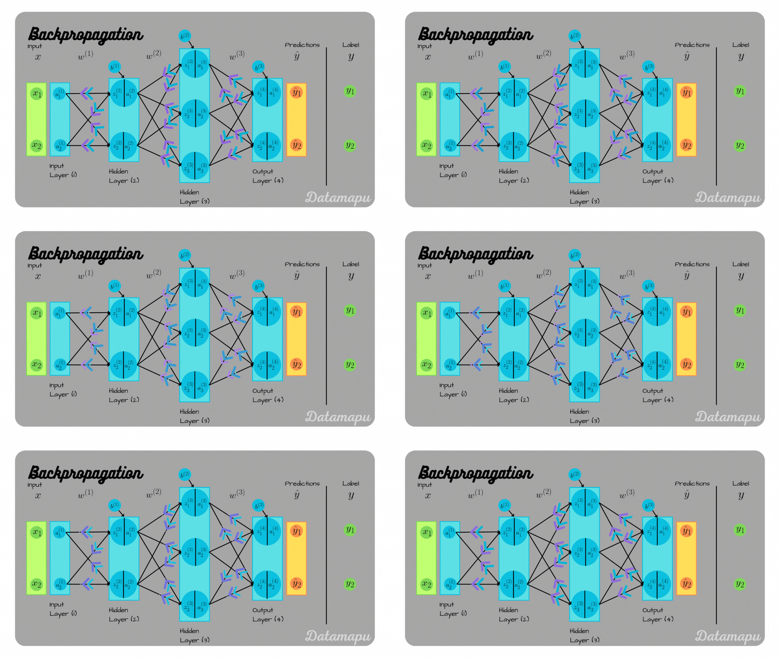
This post is quite long because of the detailed examples. If you want to skip some parts, these are the links to the examples.

• 1. Example: One Neuron
• 2. Example: Two Neurons
• 3. Example: Two Neurons in a Layer

Main Concepts of Training a Neural Net

Before starting with the first example, let’s quickly go through the main ideas of the training process of a neural net. The first thing we need, when we want to train a neural net is the training data. The training data consists of pairs of inputs and labels. The inputs are also called features and are usually written as $X = (x_1, \dots, x_n)$, with $n$ the number of data samples. The labels are the expected outcomes - or true values - and they are usually denoted as $y = (y_1, \dots, y_n)$. Training a neural net is an iterative process over a certain number of epochs. In each epoch, the training data is processed through the network in a so-called forward pass, which results in the model output. Then the error - loss - of model output compared to the true values is calculated to evaluate the model. Finally, in the backward pass - the backpropagation - Gradient Descent is used to update the model parameters and reduce the loss. Note, that in practice, generally no pure gradient descent is used, but a variant of it. We are not going into detail here, but important to understand is that some optimization algorithm is used to update the weights and biases. For a general and more detailed introduction to Deep Learning terms and concepts, please refer to Introduction to Deep Learning.

If not mentioned differently, we use the following data, activation function, and loss throughout the examples of this post.

Training Data

We consider the most simple situation with one-dimensional input data and just one sample $x = 0.5$ and labels $y = 1$.

Activation Function

As activation function, we use the Sigmoid function

$$\sigma(x) = \frac{1}{1 + e^{-x}}.$$

Loss Function

As loss function, we use the Sum of the Squared Error, defined as

$$L(y, \hat{y}) = \frac{1}{2}\sum_{p=1}^n(y_p - \hat{y}_p)^2,$$

with $y_i = (y_1, \dots, y_n)$ the labels and $\hat{y} = (\hat{y}_1, \dots, \hat{y}_n)$ the predicted labels, and $n$ the number of samples. In the examples considered in this post, we are only considering one-dimensional data, which means $n=1$ and the formula simplifies to

$$L(y, \hat{y}) = \frac{1}{2} (y - \hat{y})^2.$$

1. Example: One Neuron

To illustrate how backpropagation works, we start with the most simple neural network, which only consists of one single neuron.

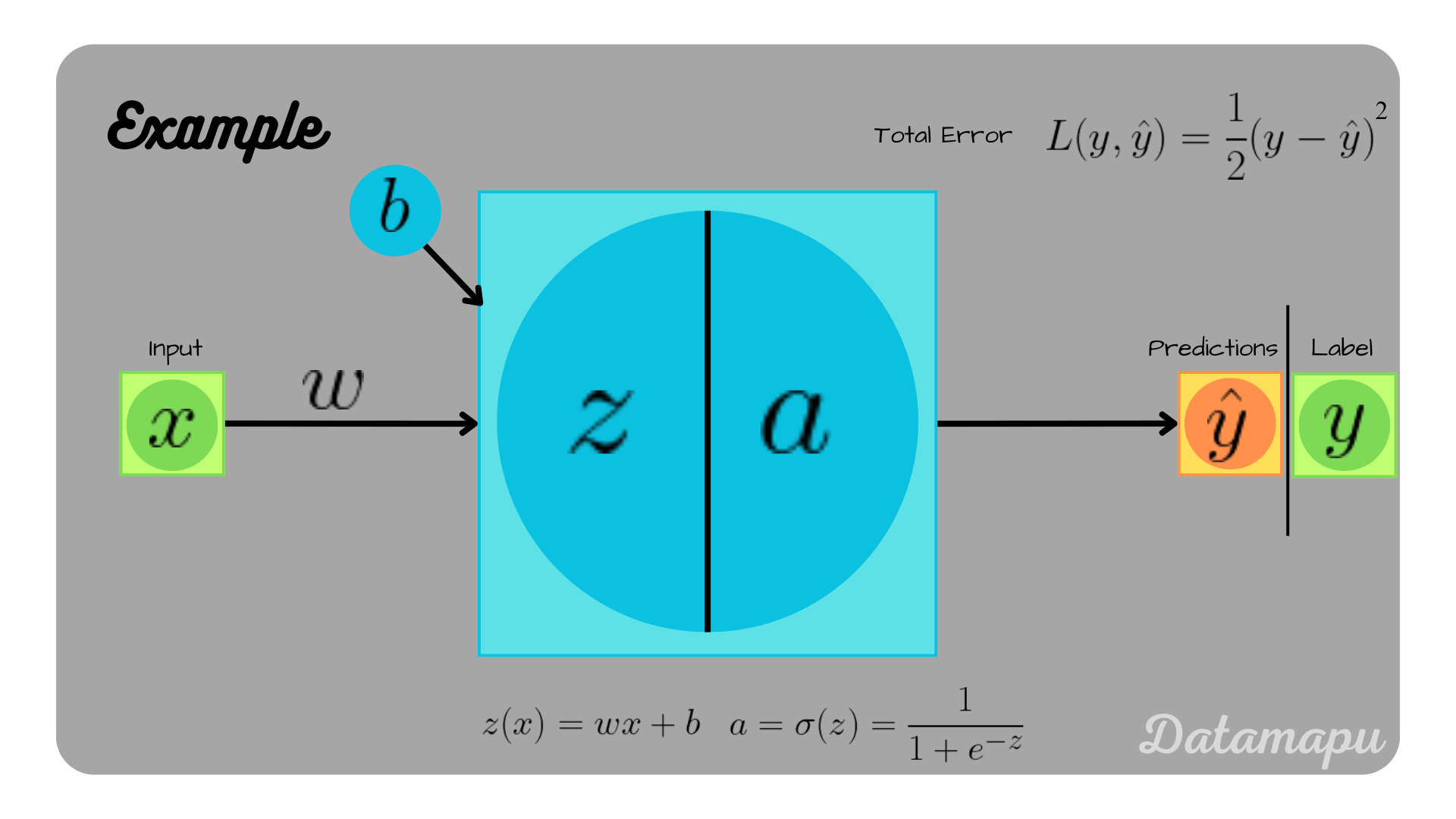Illustration of a Neural Network consisting of a single Neuron.

In this simple neural net, $z(x) = w\cdot x + b$ represents the linear part of the neuron and $a$ the activation function, which we chose to be the sigmoid function, i.e. $a = \sigma(z) = \frac{1}{1 + e^{-z}}$. For the following calculations, we assume the initial weight $w = 0.3$ and the initial bias $b = 0.1$. Further, the learning rate is set to $\alpha = 0.1$. These values are chosen arbitrarily for illustration purposes.

The Forward Pass

We can calculate the forward pass through this network as

$$\hat{y} = \sigma(z)$$ $$\hat{y} = \sigma(wx + b),$$ $$\hat{y} = \frac{1}{1 + e^{-(wx+b)}}$$.

Using the weight, and bias defined above, we get for $x = 0.5$

$$\hat{y} = \frac{1}{1 + e^{-(0.3\cdot 0.5 + 0.1)}} = \frac{1}{1 + e^{-0.25}} \approx 0.56$$

The error after this forward pass can be calculated as

$$L(1.5, 0.56) = \frac{1}{2}(1.5 - 0.56)^2 = 0.44.$$

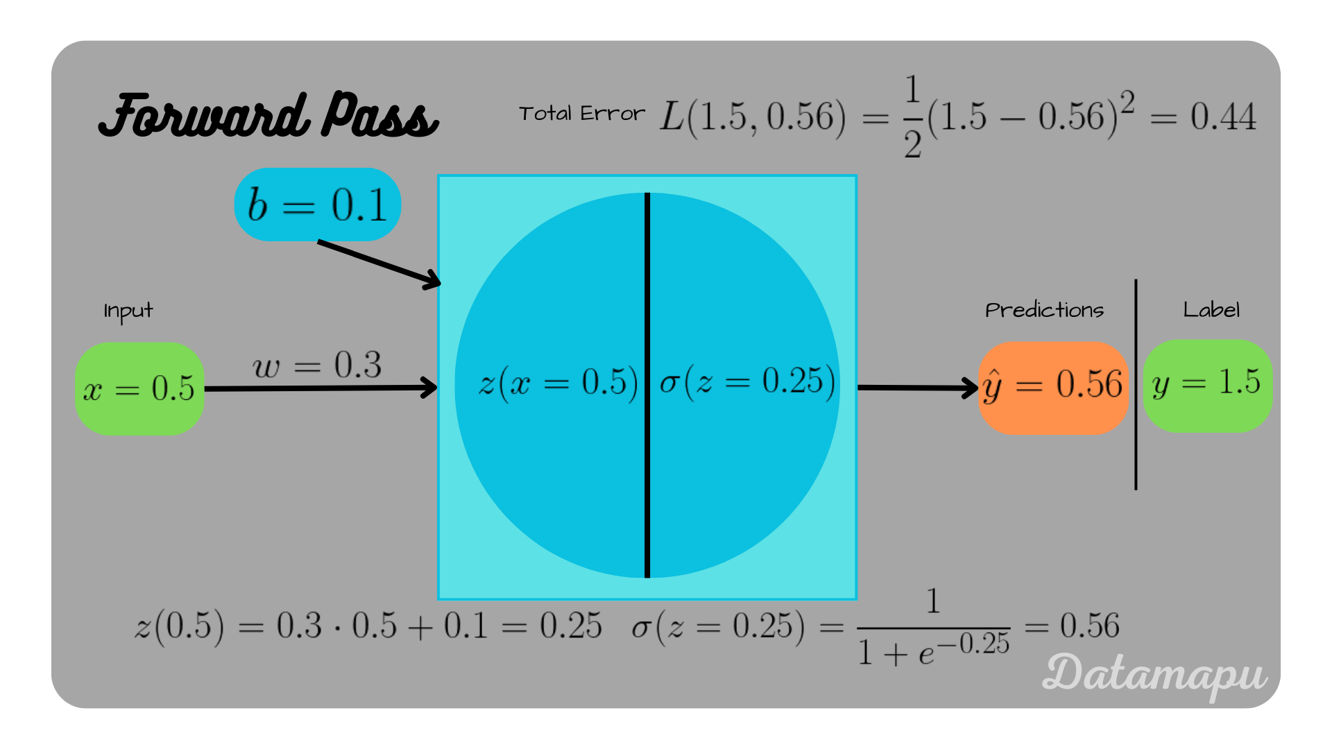Forward pass through the neural net.

The Backward Pass

To update the weight and the bias we use Gradient Descent, that is

$$w_{new} = w - \alpha \frac{\delta L}{\delta w}$$ $$b_{new} = b - \alpha \frac{\delta L}{\delta b},$$

with $\alpha = 0.1$ the learning rate. That is we need to calculate the partial derivatives of $L$ with respect to $w$ and $b$ to get the new weight and bias. This can be done using the chain rule and is illustrated in the plots below.

$$\frac{\delta L}{\delta w} = \frac{\delta L }{\delta \hat{y}} \frac{\delta \hat{y}}{\delta z} \frac{\delta z}{\delta w}$$ $$\frac{\delta L}{\delta b} = \frac{\delta L }{\delta \hat{y}} \frac{\delta \hat{y}}{\delta z} \frac{\delta z}{\delta b}$$

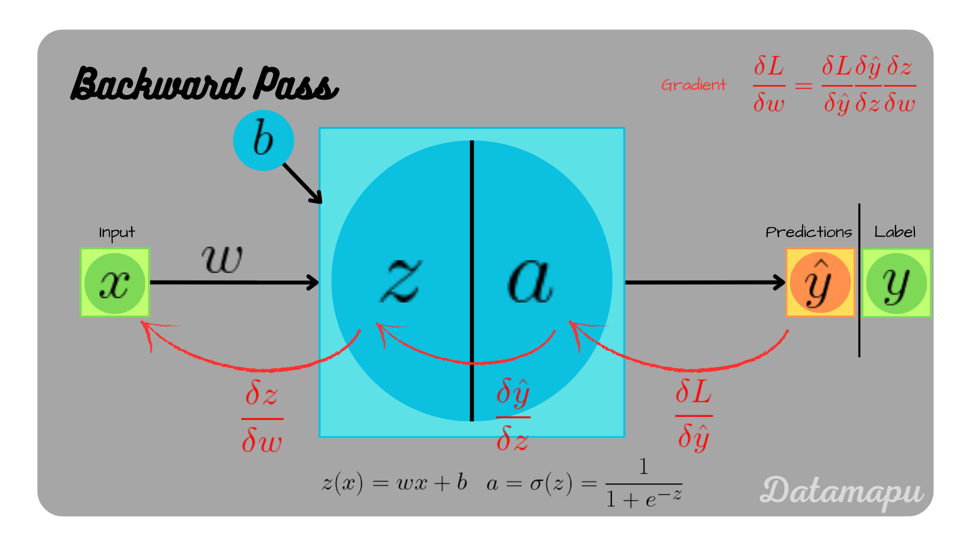
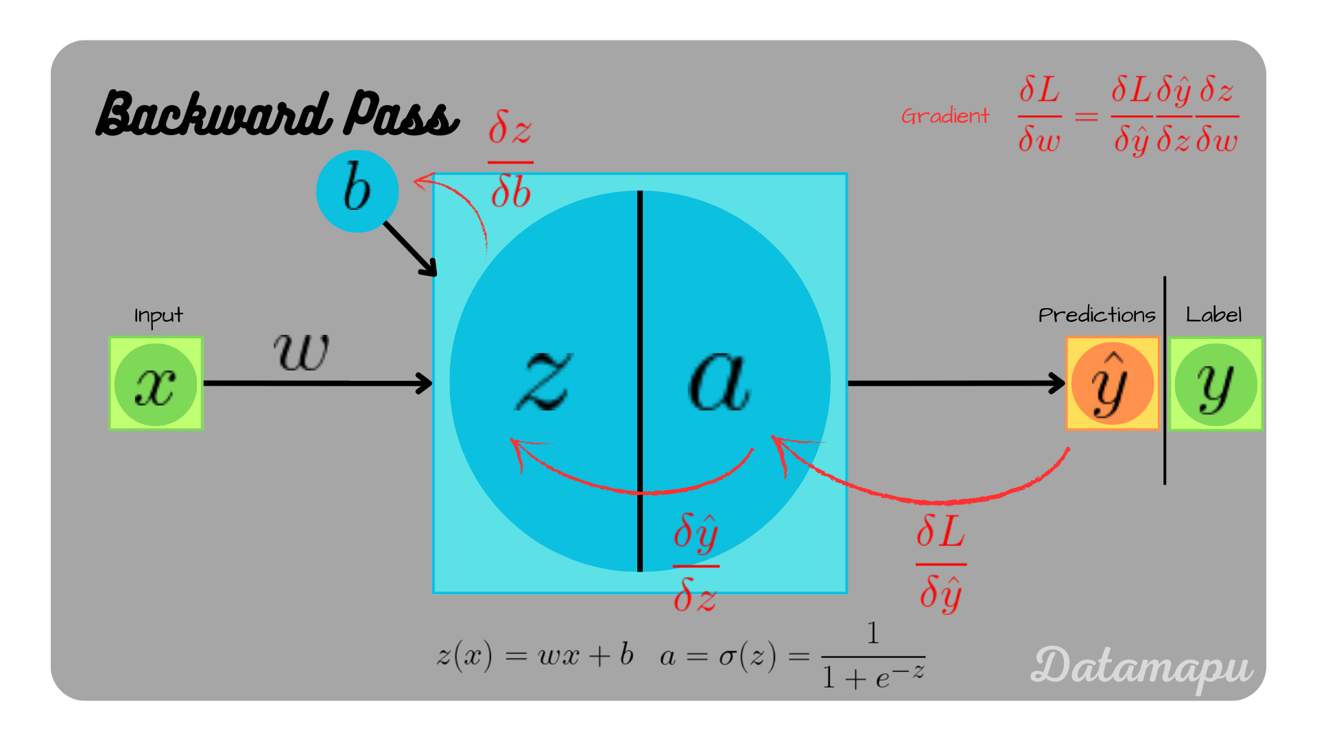Illustration of backpropagation in a neural network consisting of a single neuron.

We can calculte the individual derivatives as

$$\frac{\delta L}{\delta \hat{y}} = \frac{\delta}{\delta \hat{y}} \frac{1}{2} (y - \hat{y})^2 = - (y - \hat{y}),$$ $$\frac{\delta \hat{y}}{\delta z} = \frac{\delta}{\delta z} \sigma(z) = \sigma(z)\cdot \big(1 - \sigma(z)\big),$$ $$\frac{\delta z}{\delta w} = \frac{\delta}{\delta w} (w\cdot x + b) = x,$$ $$\frac{\delta z}{\delta b} = \frac{\delta}{\delta b} (w\cdot x + b) = 1.$$

Please find the detailed calculation of the derivative of the sigmoid function in the appendix of this post.

For the data we are considering, we get for the first equation

$$\frac{\delta L}{\delta \hat{y}} = - (y - \hat{y}) = - (1.5 - 0.56) = -0.94.$$

The second equation leads to $$\frac{\delta \hat{y}}{\delta z} = \sigma(z)\cdot \big(1 - \sigma(z)\big)$$ $$\frac{\delta \hat{y}}{\delta z} = \frac{1}{1 + e^{-0.25}}\Big( 1 - \frac{1}{1 + e^{-0.25}}\Big) = 0.56\cdot 0.44 = 0.25,$$

and finally $$\frac{\delta z}{\delta w} = x = 0.5,$$ $$\frac{\delta z}{\delta b} = 1.$$

Putting the equations back together, we get

$$\frac{\delta L}{\delta w} = -0.94 \cdot 0.25 \cdot 0.5 = -0.118$$ $$\frac{\delta L}{\delta b} = -0.94 \cdot 0.25 \cdot 1 = -0.235$$

The calculation for $\frac{\delta L }{\delta w}$ is illustrated in the plot below.

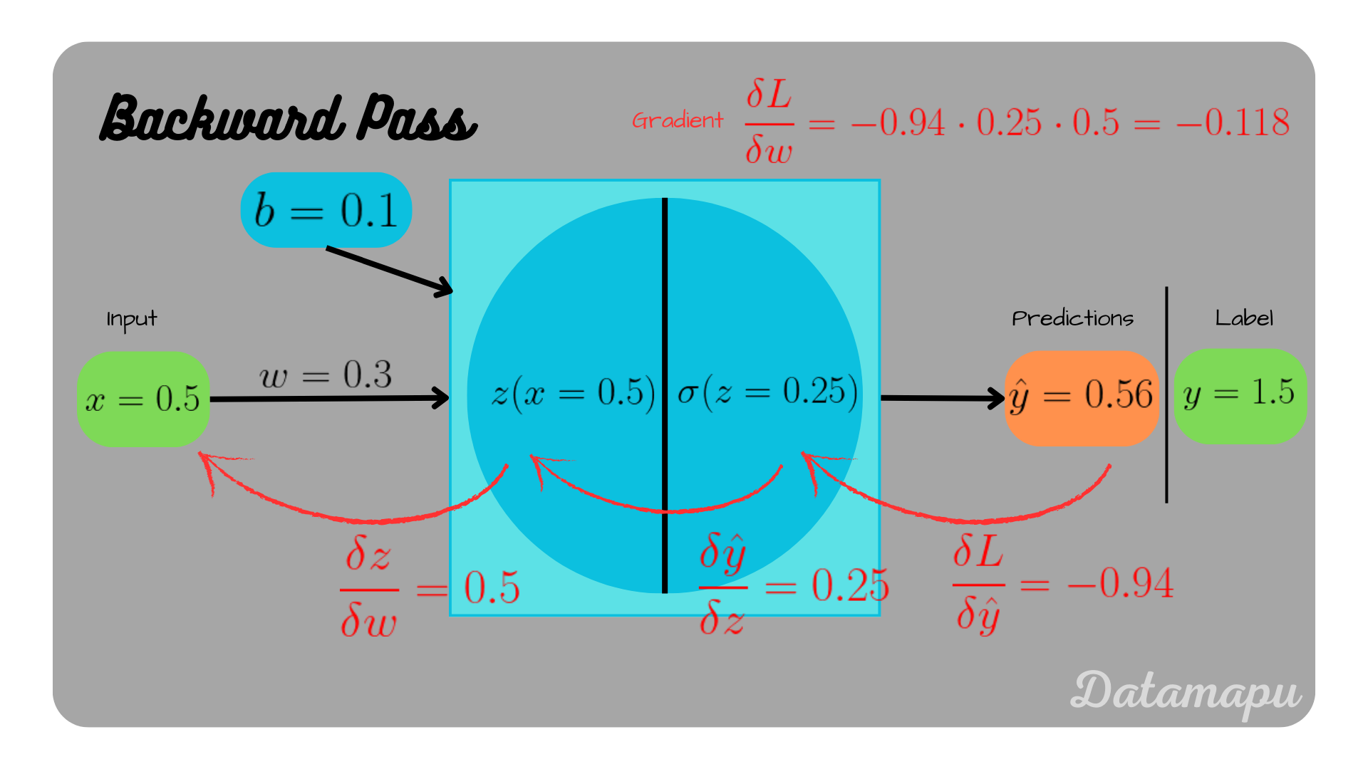Backpropagation for the weight $w$.

The weight and the bias then update to

$$w_{new} = 0.3 - 0.1 \cdot (-0.118) = 0.312,$$ $$b_{new} = 0.1 - 0.1 \cdot (-0.235) = 0.125.$$

Note

With this simple example, we illustrated one forward and one backward pass. It is a good example to understand the calculations, in real projects, however, data and neural nets are much more complex. In reality, one forward pass consists of processing all the $n$ data samples through the network, and accordingly the backward pass.

2. Example: Two Neurons

The second example we consider is a neural net, which consists of two neurons after each other, as illustrated in the following plot. Note, that the illustration is slightly different. We skipped the last arrow towards $\hat{y}$ because the second neuron’s output after applying the activation function is equal to $\hat{y}$. Also for consistency of the notation, we added $a^{(1)}$, which is equal to the input $x$. In this case we have two weights $(w^{(1)}, w^{(2)})$ and two biases $(b^{(1)}, b^{(2)})$. We set $w^{(1)} = 0.3$, $w^{(2)} = 0.2$, $b^{(1)} = 0.1$, and $b^{(2)} = 0.4$. As in the first example, these numbers are chosen arbitrarily.

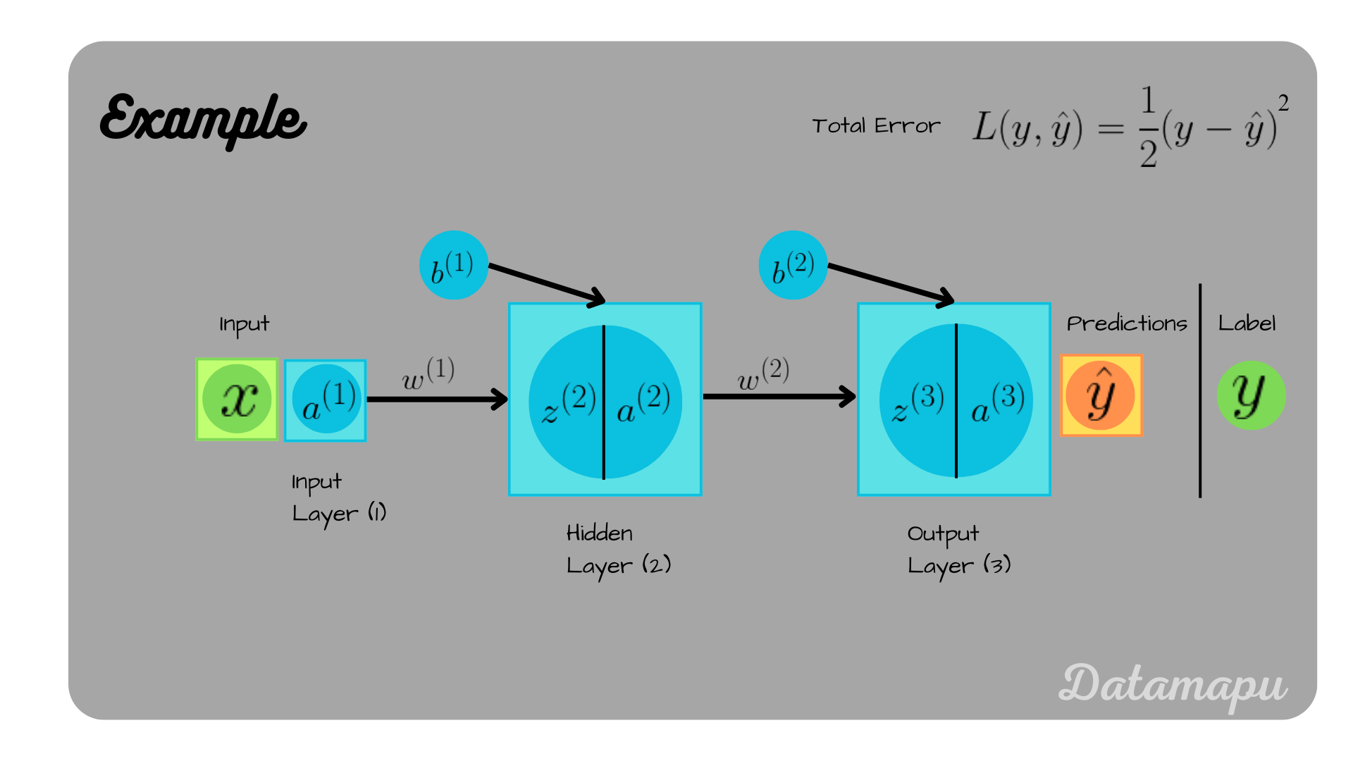A neural net with two layers, each consisting of one neuron.

The Forward Pass

The forward pass is calculated as follows

$$\hat{y} = a^{(3)} = \sigma(z^{(3)}) = \sigma(w^{(2)} a^{(2)} + b^{(2)}),$$ with $$a^{(2)} = \sigma(z^{(2)}) = \sigma(w^{(1)} a^{(1)} + b^{(1)}) = \sigma(w^{(1)} x + b^{(1)}).$$

Together this leads to

$$\hat{y} = \sigma\big(w^{(2)}\cdot \sigma(w^{(1)} \cdot x + b^{(1)}) + b^{(2)}\big).$$

Using the values define above, we get

$$\hat{y} = \sigma\Big(0.2\cdot \big(\sigma(0.3 \cdot 0.5 + 0.1)\big) + 0.4\Big) = \sigma\big(0.2\cdot \sigma(0.25) + 0.4\big)$$ $$\hat{y} = \sigma\big(0.2\cdot \frac{1}{1 + e^{-0.25}} +0.4\big) \approx \sigma(0.2\cdot 0.56 + 0.4)$$ $$\hat{y} \approx \sigma(0.512) = \frac{1}{1 + e^{-0.512}} = 0.625.$$

The loss in this case is

$$L(y, \hat{y}) = \frac{1}{2} (1.5 - 0.625)^2 = 0.38.$$

The Backward Pass

In the backward pass, we want to update all the four model parameters - the two weights and the two biases.

$$w^{(1)}_{new} = w^{(1)} - \alpha \frac{\delta L}{\delta w^{(1)}}$$

$$b^{(1)}_{new} = b^{(1)} - \alpha \frac{\delta L}{\delta b^{(1)}}$$

$$w^{(2)}_{new} = w^{(2)} - \alpha \frac{\delta L}{\delta w^{(2)}}$$

$$b^{(2)}_{new} = b^{(2)} - \alpha \frac{\delta L}{\delta b^{(2)}}$$

For $w^{(2)}$ and $b^{(2)}$, the calculations are analogue to the ones in the first example. Following the steps shown above, we get

$$\frac{\delta L}{\delta w^{(2)}} = \frac{\delta L}{\delta \hat{y}} \frac{\delta \hat{y}}{\delta z^{(3)}} \frac{\delta z^{(3)}}{\delta w^{(2)}} = (-0.875) \cdot 0.235 \cdot 0.5 = -0.103$$

$$\frac{\delta L}{\delta b^{(2)}} = \frac{\delta L}{\delta \hat{y}} \frac{\delta \hat{y}}{\delta z^{(3)}} \frac{\delta z^{(3)}}{\delta b^{(2)}} = (-0.875)\cdot 0.235 = -0.205$$

We will now focus on the remaining two. The idea is exactly the same, only we now have to apply the chain-rule several times

$$\frac{\delta L}{\delta w^{(1)}} = \frac{\delta L}{\delta \hat{y}} \frac{\delta \hat{y}}{\delta z^{(3)}} \frac{\delta z^{(3)}}{\delta a^{(2)}} \frac{\delta a^{(2)}}{\delta z^{(2)}} \frac{\delta z^{(2)}}{\delta w^{(1)}},$$

and

$$\frac{\delta L}{\delta b^{(1)}} = \frac{\delta L}{\delta \hat{y}} \frac{\delta \hat{y}}{\delta z^{(3)}} \frac{\delta z^{(3)}}{\delta a^{(2)}} \frac{\delta a^{(2)}}{\delta z^{(2)}} \frac{\delta z^{(2)}}{\delta b^{(1)}},$$

as illustrated in the following plots.

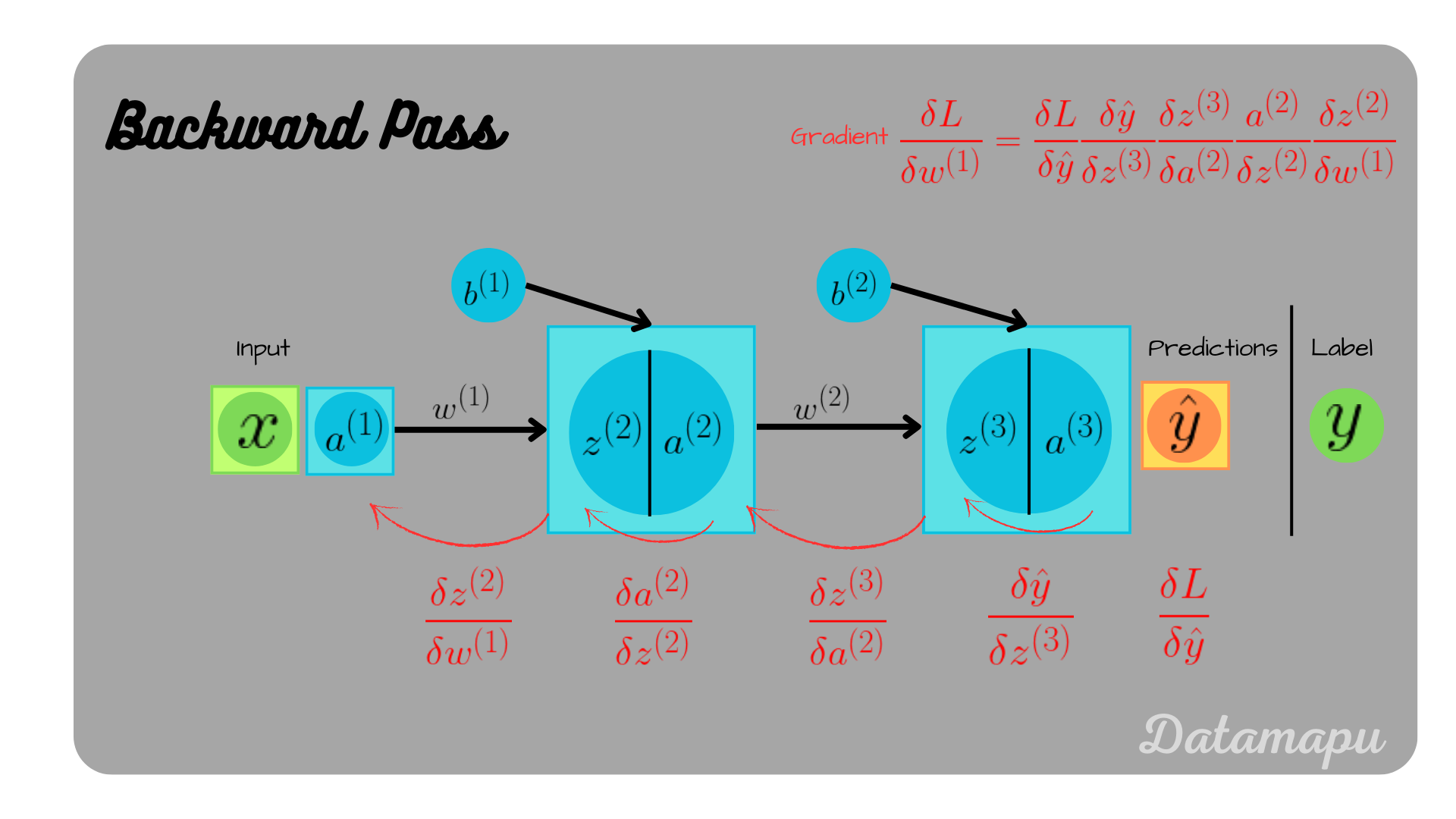
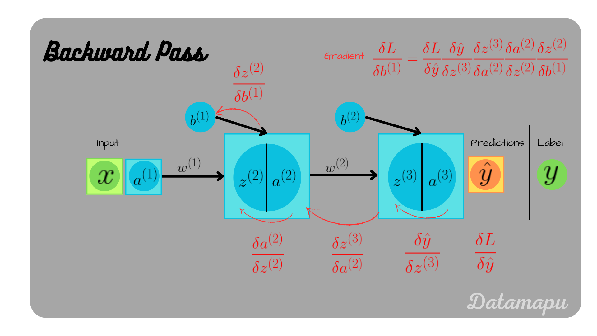Backpropagation illustrated.

Calculting the individual derivatives, we get

$$\frac{\delta L}{\delta \hat{y}} = -(y - \hat{y})$$

$$\frac{\delta \hat{y}}{\delta z^{(3)}} = \frac{\delta}{\delta z^{(3)}} \sigma(z^{(3)}) = \sigma(z^{(3)}) \big(1- \sigma(z^{(3)})\big)$$

$$\frac{\delta z^{(3)}}{\delta a^{(2)}} = \frac{\delta}{\delta a^{(2)}}w^{(2)} a^{(2)} + b^{(2)} = w^{(2)}$$

$$\frac{\delta a^{(2)}}{\delta z^{(2)}} = \frac{\delta}{\delta z^{(2)}} \sigma(z^{(2)}) = \sigma(z^{(2)}) \big(1- \sigma(z^{(2)})\big)$$

$$\frac{\delta z^{(2)}}{\delta w^{(1)}} = \frac{\delta}{\delta w^{(1)}}w^{(1)} x + b^{(1)} = a^{(1)}$$

$$\frac{\delta z^{(2)}}{\delta b^{(1)}} = \frac{\delta}{\delta b^{(1)}}w^{(1)} x + b^{(1)} = 1$$

For the detailed development of the derivative of the sigmoid function, please check the appendix of this post. With the values defined, we get for the first equation

$$\frac{\delta L}{\delta \hat{y}} = -(y - \hat{y}) = -(1.5 - 0.625) = -0.875.$$

For the second equation

$$\frac{\delta \hat{y}}{\delta z^{(3)}} = \sigma(z^{(3)}) \big(1- \sigma(z^{(3)})\big),$$

with $z^{(3)}$ calculated as

$$z^{(3)} = w^{(2)} a^{(2)} + b^{(2)} = \sigma(w^{(1)} a^{(1)} + b^{(1)}) = \sigma(w^{(1)} x + b^{(1)}) = \sigma(0.25) \approx 0.56,$$

we get

$$\frac{\delta \hat{y}}{\delta z^{(3)}} = \frac{1}{1 + e^{-0.56}}\big(1 - \frac{1}{1 + e^{-0.56}}\big) \approx 0.64 \cdot (1 - 0.64) = 0.23.$$

For the third equation, we get

$$\frac{\delta z^{(3)}}{\delta a^{(2)}} = w^{(2)} = 0.2$$

The fourth equation leads to

$$\frac{\delta a^{(2)}}{\delta z^{(2)}} = \sigma(z^{(2)}) \big(1- \sigma(z^{(2)})\big),$$

with

$$z^{(2)} = w^{(1)} a^{(1)} + b^{(1)} = w^{(1)} x + b^{(1)} = 0.3\cdot 0.5 + 0.1 = 0.25.$$

Replacing this in the above equation leads to

$$\frac{\delta a^{(2)}}{\delta z^{(2)}} = \sigma(0.25) \big(1 - \sigma(0.25)\big) \approx 0.56 \cdot (1 - 0.56) \approx 0.25,$$

The fifth equation gives

$$\frac{\delta z^{(2)}}{\delta w^{(1)}} = x = 0.5,$$

and the last equation is always equal to $1$.

Putting the derivatives back together, we get

$$\frac{\delta L}{\delta w^{(1)}} = (-0.875)\cdot 0.23 \cdot 0.2 \cdot 0.25 \cdot 0.5 \approx -0.005,$$

and

$$\frac{\delta L}{\delta b^{(1)}} = (-0.875)\cdot 0.23 \cdot 0.2 \cdot 0.25 \cdot 1 \approx -0.01$$

With that we can update the weights

$$w^{(1)}_{new} = 0.3 - 0.1 \cdot (-0.005) = 0.3005$$

$$b^{(1)}_{new} = 0.1 - 0.1 \cdot (-0.01) = 0.101$$

$$w^{(2)}_{new} = 0.2 - 0.1 \cdot (-0.103) = 0.2103$$

$$b^{(2)}_{new} = 0.4 - 0.1 \cdot (-0.205) = 0.3795$$

3. Example: Two Neurons in a layer

In this example, we will consider a neural net, that consists of two neurons in the hidden layer. We are not going to cover it in detail, but we will have a look at the equations that need to be calculated. For illustration purposes, the bias term is illustrated as one vector for each layer, i.e. in the below plot $b^{(1)} = (b^{(1)}_1, b^{(1)}_2)$ and $b^{(2)} = (b^{(2)}_1, b^{(2)}_2)$.

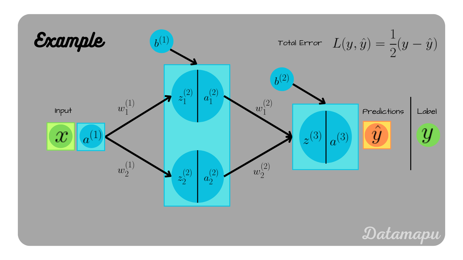Example with two neurons in one layer.

Forward Pass

In the forward pass we now have to consider the sum of the two neurons in the layer. It is calculated as

$$\hat{y} = a^{(3)} = \sigma(z^{(3)}) = \sigma\big(w^{(2)}_1\cdot a^{(2)}_1 + b^{(2)}_1 + w^{(2)}_2 \cdot a^{(2)}_2 + b^{(2)}_2\big),$$

with

$$a^{(2)}_1 = \sigma(z^{(2)}_1) = \sigma\big(a^{(1)}_1 x + b^{(1)}_1 \big) = \frac{1}{1 + e^{-(a^{(1)}_1 x + b^{(1)}_1)}},$$

$$a^{(2)}_1 = \sigma(z^{(2)}_2) = \sigma\big(a^{(1)}_2 x + b^{(1)}_2 \big) = \frac{1}{1 + e^{-(a^{(1)}_2 x + b^{(1)}_2)}},$$

this leads to

$$\hat{y} = \frac{1}{1 + e^{-(w^{(2)}_1\cdot a^{(2)}_1 + b^{(2)}_1 + w^{(2)}_2 \cdot a^{(2)}_2 + b^{(2)}_2)}}$$ $$\hat{y} = \frac{1}{1 + e^{-\Big(w^{(2)}_1\cdot \Big(\frac{1}{1 + e^{-(a^{(1)}_1 x + b^{(1)}_1)}}\Big) + b^{(2)}_1 + w^{(2)}_2 \cdot \Big(\frac{1}{1 + e^{-(a^{(1)}_2 x + b^{(1)}_2)}}\Big) + b^{(2)}_2)\Big)}},$$

with

$$a_i^{(1)} = w_{i1}^{(2)}\cdot a_1^{(2)} + b_1^{(2)} + w_{i2}^{(2)}\cdot a_2^{(2)} + b_2^{(2)} $$

for $i = 1, 2$.

Backward Pass

For the backward pass we need to calculate the partial derivatives as follows

$$w^{(1)}_{1,new} = w^{(1)}_1 - \alpha \frac{\delta L}{\delta w^{(1)}_1}$$

$$w^{(1)}_{2,new} = w^{(1)}_2 - \alpha \frac{\delta L}{\delta w^{(1)}_2}$$

$$b^{(1)}_{1,new} = b^{(1)} - \alpha \frac{\delta L}{\delta b^{(1)}_1}$$

$$b^{(1)}_{2,new} = b^{(1)} - \alpha \frac{\delta L}{\delta b^{(1)}_2}$$

$$w^{(2)}_{1,new} = w^{(1)}_1 - \alpha \frac{\delta L}{\delta w^{(2)}_1}$$

$$w^{(2)}_{2,new} = w^{(1)}_2 - \alpha \frac{\delta L}{\delta w^{(2)}_2}$$

$$b^{(2)}_{1,new} = b^{(2)}_1 - \alpha \frac{\delta L}{\delta b^{(2)}_1}$$

$$b^{(2)}_{2,new} = b^{(2)}_2 - \alpha \frac{\delta L}{\delta b^{(2)}_2}$$

We can calculate all the partial derivatives as shown in the above two examples. The calculations for $\frac{\delta L}{\delta w^{(2)}_1}$, $\frac{\delta L}{\delta w^{(2)}_2}$, and $\frac{\delta L}{\delta b^{(2)}}$ are as the ones shown in the first example. Further $\frac{\delta L}{\delta w^{(1)}_1}$, $\frac{\delta L}{\delta b^{(1)}_2}$, $\frac{\delta L}{\delta w^{(b)}_1}$, and $\frac{\delta L}{\delta w^{(2)}_2}$ are calculated analgue to example 2. The calculations of the latter are illustrated in the below plot.

$$\frac{\delta L}{\delta w^{(1)}_1} = \frac{\delta L}{\delta \hat{y}} \frac{\delta \hat{y}}{\delta z^{(3)}} \frac{\delta z^{(3)}}{\delta a^{(2)}_1} \frac{\delta a^{(2)}_1}{\delta z^{(2)}_1} \frac{\delta z^{(2)}_1}{\delta w^{(1)}_1},$$

$$\frac{\delta L}{\delta w^{(1)}_2} = \frac{\delta L}{\delta \hat{y}} \frac{\delta \hat{y}}{\delta z^{(3)}} \frac{\delta z^{(3)}}{\delta a^{(2)}_1} \frac{\delta a^{(2)}_1}{\delta z^{(2)}_1} \frac{\delta z^{(2)}_1}{\delta w^{(1)}_2},$$

$$\frac{\delta L}{\delta b^{(1)}_1} = \frac{\delta L}{\delta \hat{y}} \frac{\delta \hat{y}}{\delta z^{(3)}} \frac{\delta z^{(3)}}{\delta a^{(2)}_1} \frac{\delta a^{(2)}_1}{\delta z^{(2)}_1} \frac{\delta z^{(2)}_1}{\delta b^{(1)}_1},$$

$$\frac{\delta L}{\delta b^{(1)}_2} = \frac{\delta L}{\delta \hat{y}} \frac{\delta \hat{y}}{\delta z^{(3)}} \frac{\delta z^{(3)}}{\delta a^{(2)}_1} \frac{\delta a^{(2)}_1}{\delta z^{(2)}_1} \frac{\delta z^{(2)}_1}{\delta b^{(1)}_2},$$

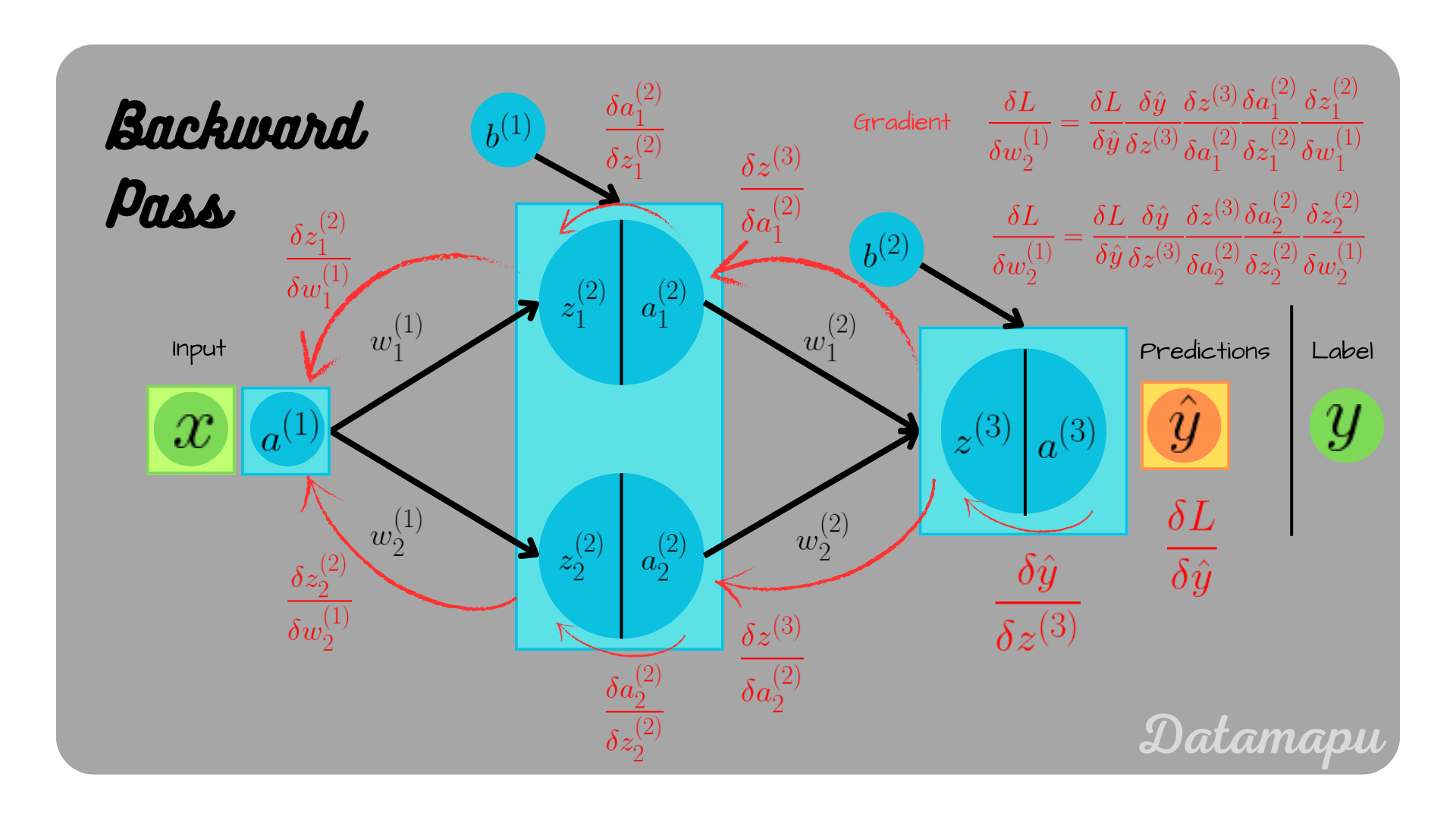Backpropagation illustrated for the weights.

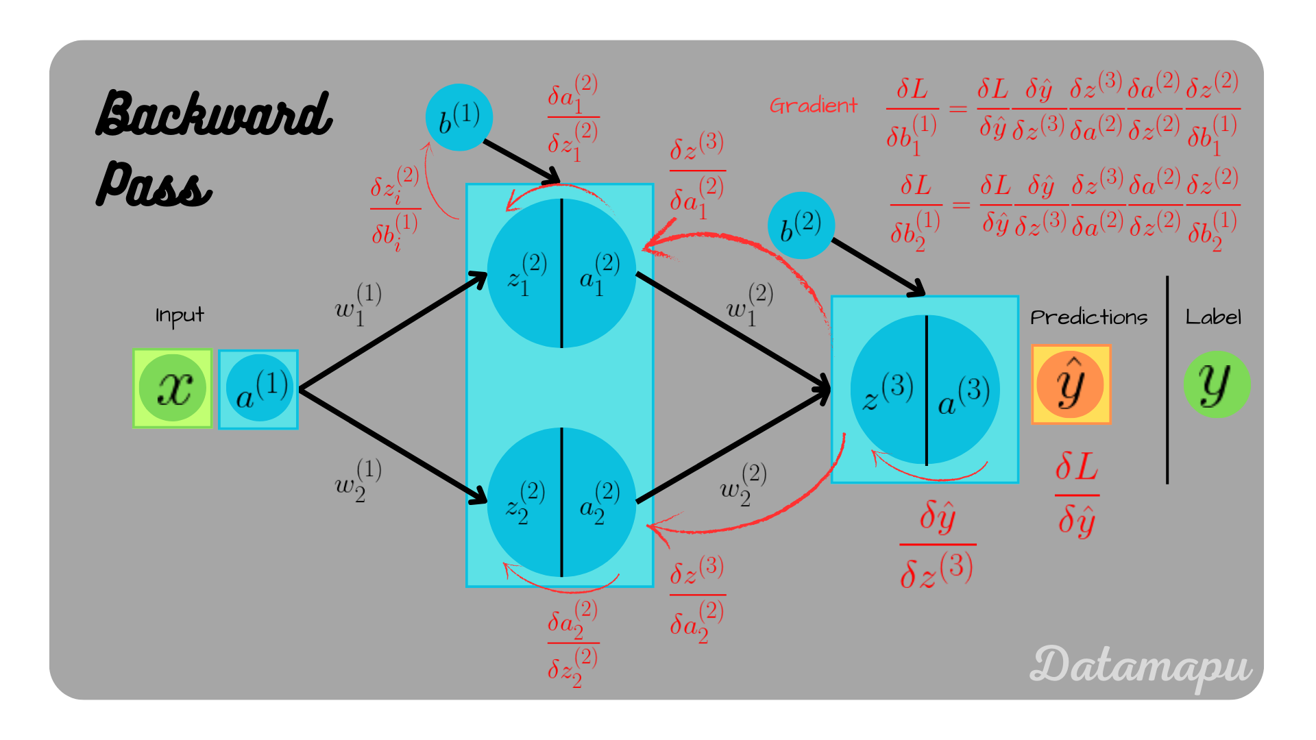Backpropagation illustrated for the biases.

We can see that even for this very small and simple neural net, the calculations easily get overwhelming.

Note

In the above considered examples the data used was one-dimensional, which makes the calculations easier. If the output has $n>1$ dimensions, the loss function becomes a sum

$$L(y, \hat{y}) = \frac{1}{2}\sum_{p=1}^n(y_p - \hat{y}_p)^2.$$

The partial derivative of $L$ can then be written as

$$\frac{\delta L}{\delta w_{ij}^{(k)}} = \sum_{p=1}^n \frac{\delta L_p}{\delta w_{ij}^{(k)}},$$

with

$$L_p = \frac{1}{2}(y_p - \hat{y}_p)^2.$$

Summary

To train a neural network the weights and biases need to be optimized. This is done using backpropagation. In this post we calculated the backpropagation algorithm for some simplified examples in detail. Gradient Descent is used to update the model parameters. The general concept of calculating the gradient is calculating the partial derivatives of the loss function using the chain rule.

Further Reading

More general formulations of the backpropagation algorithm can be found in the following links.

• Wikipedia
• Neural Networks and Deep Learning - How the backpropagation algorithm works, Michael Nielsen
• Brilliant - Backpropagation
• Backpropagation, Jorge Leonel

Appendix

Derivative of the Sigmoid Functioni

The Sigmoid Function is defined as

$$\sigma(x) = \frac{1}{1 + e^{-x}}$$

The derivative can be derived using the chain rule

$$\sigma\prime(x) = \frac{\delta}{\delta x} \sigma(x) = \frac{\delta}{\delta x} (1 + e^{-x})^{-1} = -(1 + e^{-x})^{-2} \frac{\delta}{\delta x}(1 + e^{-x}).$$

In the last expression we applied the outer derivative, calculating the inner derivative again needs the chain rule.

$$\sigma\prime(x) = -(1 + e^{-x})^{-2} e^{-x} \cdot (-1).$$

This can be reformulated to

$$\sigma\prime(x) = \frac{e^{-x}}{(1 + e^{-x})^2}$$ $$\sigma\prime(x) = \frac{e^{-x}}{(1 + e^{-x})(1 + e^{-x})}$$ $$\sigma\prime(x) = \frac{1}{1 + e^{-x}} \cdot \frac{e^{-x}}{1 + e^{-x}}$$ $$\sigma\prime(x) = \frac{1}{1 + e^{-x}} \cdot \frac{e^{-x} + 1 - 1}{1 + e^{-x}}$$ $$\sigma\prime(x) = \frac{1}{1 + e^{-x}} \cdot \big(\frac{1 + e^{-x}}{1 + e^{-x}} - \frac{1}{1 + e^{-x}} \big)$$ $$\sigma\prime(x) = \frac{1}{1 + e^{-x}} \cdot \big(1 - \frac{1}{1 + e^{-x}}\big).$$

That is, we can write the derivative as follows $$\sigma\prime(x) = \sigma(x)\cdot(1 - \sigma(x)).$$

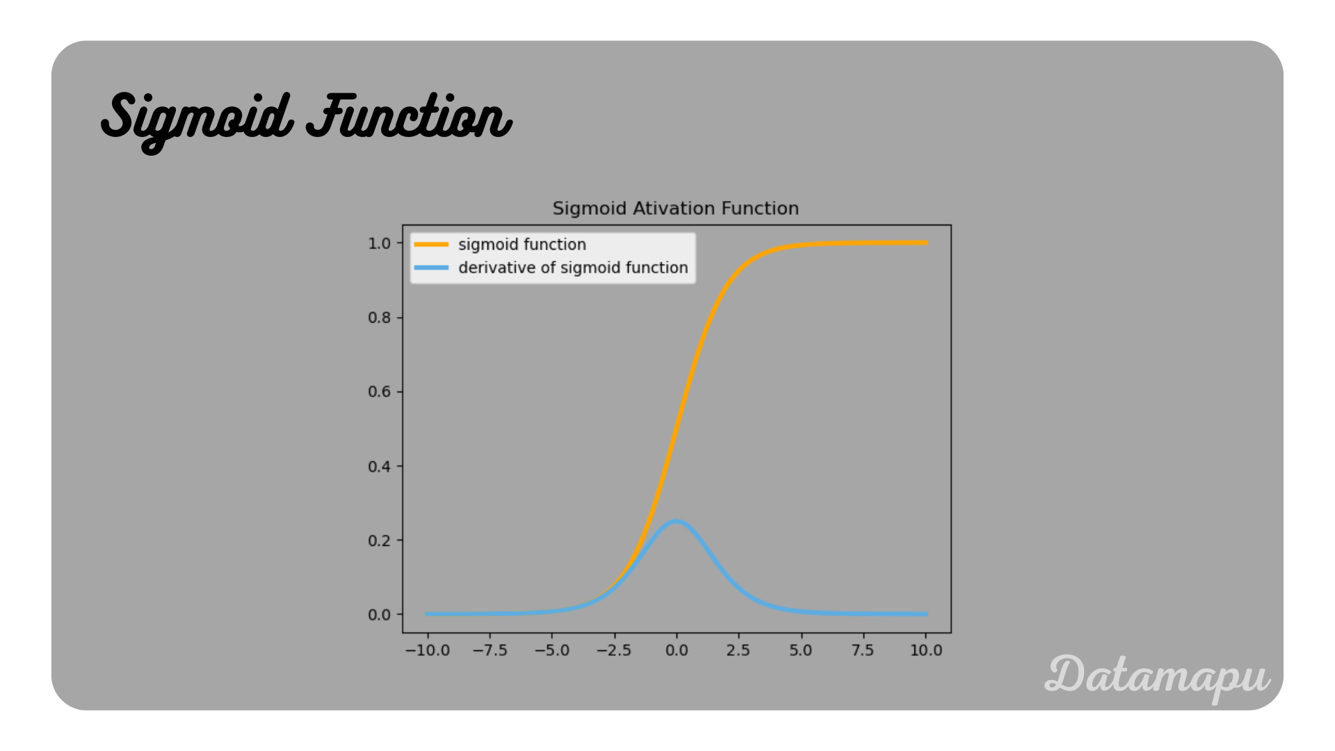Illustration of the Sigmoid function and its derivative.

If this blog is useful for you, please consider supporting.

• Backpropagation
• Data Science
• Machine Learning
• Artificial Intelligence
• Deep Learning