Gradient Descent

February 27, 2024 - 8 minutes read - 1649 words

Introduction

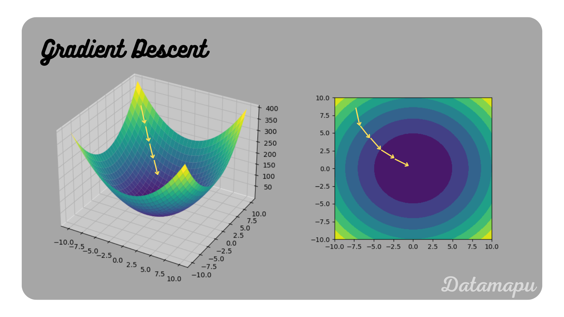
Gradient Descent is a mathematical optimization technique, which is used to find the local minima of a function. In Machine Learning it is used in a variety of models such as Gradient Boosting or Neural Networks to minimize the Loss Function. It is an iterative algorithm that takes small steps towards the minimum in every iteration. The idea is to start at a random point and then take a small step into the direction of the steepest descent of this point. Then take another small step in the direction of the steepest descent of the next point and so on. The direction of the steepest descent is determined using the gradient of the function, so its name Gradient Descent.

gradient_descent Gradient Descent illustrated.

Intuition

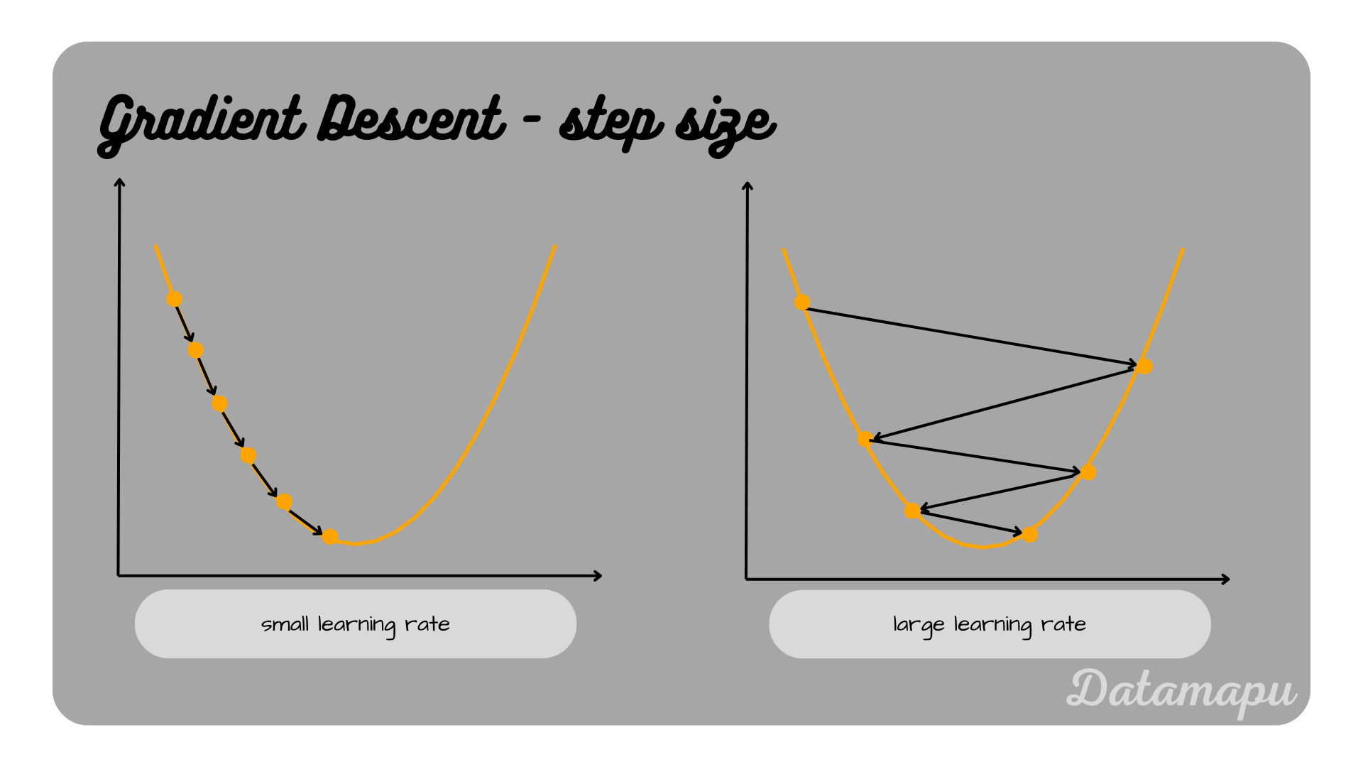
Gradient Descent is often compared to descending from the top of a mountain to a valley. To reach the valley, we take individual steps. After each step, we check which is the direction of the steepest descent for the next step and move in this direction. The step size we take may vary and affects how long we need to reach the minimum and if we reach it at all. Very small steps mean that it will take very long to get to the valley. However, if the steps are too large, especially close to the minimum, we may miss it by taking a step over it.

gradient_descent Gradient Descent intuition.

Definition

Gradient Descent is an iterative method that aims to find the minimum of a differentiable function. In the context of Machine Learning, this is usually the loss function $L = L (w_{i})$ , which depends on the model parameters. To find a local minimum, we start at an arbitrary random point and move in the direction of the steepest descent at this point. Mathematically, the direction of the steepest ascent at a specific point is defined by the gradient at this point, which is also called the slope. Consequently, the direction of the steepest descent at a point is the negative of the gradient at this point. Taking this small step we reach a new point on our loss function. At this next point, we again move a small step into the direction of the negative of the gradient. In this way, we iteratively approach the minimum. This procedure can be formulated as

$w_{i + 1} = w_{i} - α \cdot \nabla_{w_{i}} L (w_{i}),$

with $α$ the step size we take into the direction of the negative of the gradient. $α$ is a hyperparameter, which is called the learning rate. How big the learning rate is influences the convergence of the algorithm. If the learning rate is very low, a lot of iterations are needed to get to the minimum. On the other hand, if the learning rate is too large, we may overpass the minimum. One possibility is to start with a larger learning rate and make it smaller over time. Gradient Descent does not guarantee to reach a local or even global minimum. It is only certain to approach a stationary point that satisfies $\nabla_{w_{i}} L (w_{i}) = 0$ .

gradient_descent Small and large learning rate illustrated.

Variants of Gradient Descent

Batch Gradient Descent

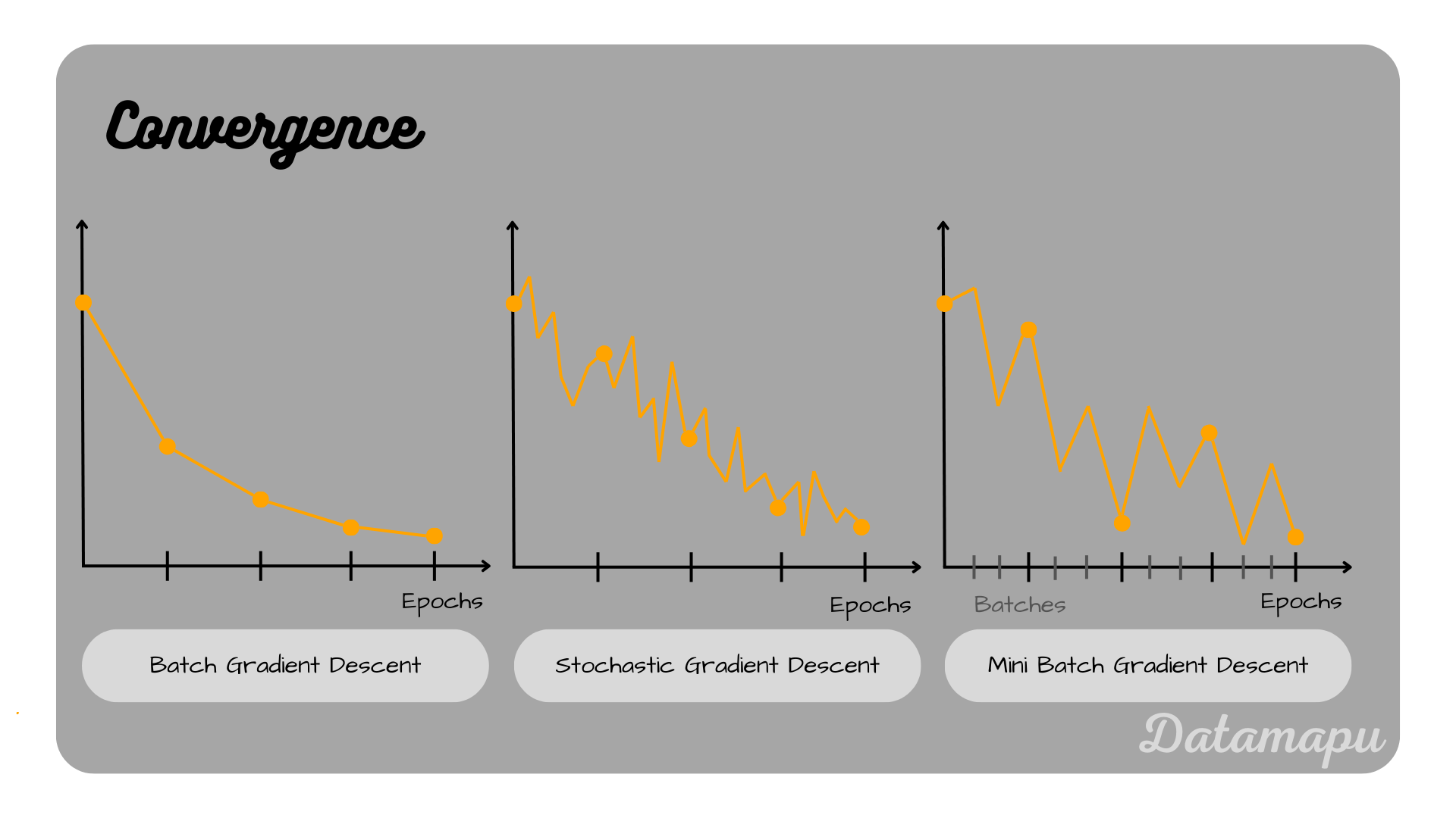
In the previous definition, we didn’t talk about how to apply Gradient Descent in practice. When we train a Neural Net we have a defined training dataset, which we train for a certain number of epochs. Training for one epoch means that the entire training dataset was processed by the Neural Network (forward and backward pass) once. The most classical variant of Gradient Descent is also sometimes called Batch Gradient Descent. In this case, the entire training dataset is processed by a forward pass through the Neural Net. Then the gradients of the loss function of all samples from the training dataset are calculated. The weights $w_{i + 1}$ are then updated using the mean of the Gradients of the entire training dataset. Since the entire training data was used, the model was trained for one epoch after applying Gradient Descent once. This strategy gives the most accurate estimate of the direction of the minimum, is however cost intensive. In pseudocode, this can be written as

for m in range(nr of epochs):
	calculate the derivative of the loss function for all samples in the dataset
	take the mean of all these derivatives
	update the weights w = w - learning rate * mean of all derivatives

Stochastic Gradient Descent

In Stochastic Gradient Descent, the samples of the training data are considered individually. For each sample the gradient is calculated and this gradient is used to update the weights. If the training data consists of $N$ samples, $N$ updates of the weights are done until the model is trained for one epoch. That means the individual step to update the weights is much faster, the accuracy however reduces and the convergence is slow. Stochastic Gradient Descent can be formulated as

$w_{i + 1} = w_{i} - α \cdot \nabla_{w_{i}} L (x^{i}, y^{i}, w_{i}) .$

The difference to the above formulation of (Batch-)Gradient Descent is that in this case, the gradient depends on the individual input $x^{i}$ and target data points $y^{i}$ . In pseudocode Stochastic Gradient Descent can be written as

for m in range(nr of epochs):
	for n in range(nr of training samples):
        	calculate the derivative of the loss function for each sample n
        	update the weights w = w - learning rate * derivative of sample n

Mini-Batch Gradient Descent

Mini-Batch Gradient Descent is a compromise of the above two variants and is very commonly used. In this case, a subset (Mini-Batch) is used and processed through the Neural Network. The gradients of these mini-batches are then calculated and the mean is taken to update the weight. Then the next mini-batch is processed through the forward pass of the Neural Net and the mean of the gradient is used to update the weight. This process is repeated until the entire dataset is used, then the Neural Net has been trained for one epoch. Common mini-batch sizes ( $b$ ) are powers of $2$ , like $b = 16, 32, 64, \dots$ . In this case, the model was trained for one epoch after $\frac{N}{b}$ updates, if $N$ is the number of training samples. The number of batches needed to complete one training epoch is called iterations. mini-batch Gradient Descent can be formulated as

$w_{i + 1} = w_{i} - α \cdot \nabla_{w_{i}} L (x^{i, i + b}, y^{i, i + b}, w_{i}) .$

In this case, the gradient depends on the batch size $b$ . Gradient Descent is thus Mini-Batch Gradient Descent, with the batch size $b$ equal to the size of the entire dataset $N$ . In pseudocode Mini-Batch Gradient Descent can be written as

for m in range(nr of epochs):
	for b in range(nr of batches):
        	calculate the derivative of the loss function for all samples in the batch
        	take the mean of all these derivatives
        	update the weights w = w - learning rate * mean of all derivatives

Illustration of the Convergence for (Batch) Gradient Descent, Stochastic Gradient Descent, and Mini-Batch Gradient Descent.

Vanishing / Exploding Gradients

When training a Neural Net, Gradient Descent is used in backpropagation to optimize the weights and biases. The phenomenon of Vanishing Gradients refers to the scenario in which the gradient gets very small until it almost vanishes. In this case, the Neural Net is not able to learn anymore, because the gradient is used to update the weights and biases. If the gradient approaches zero, no update is happening. On the other hand, the phenomenon of Exploding Gradients refers to the scenario that the gradients keep growing while they are passing backward through the Neural Net.

In backpropagation, the gradient of the loss function with respect to the weights (and biases) is calculated. For that, the partial derivatives of the loss function with respect to each weight need to be calculated using the chain rule

$\frac{δ L (w_{i})}{δ w_{i}} = \frac{δ L (\hat{y})}{δ \hat{y}} \cdot \frac{δ \hat{y}}{δ w_{i}},$

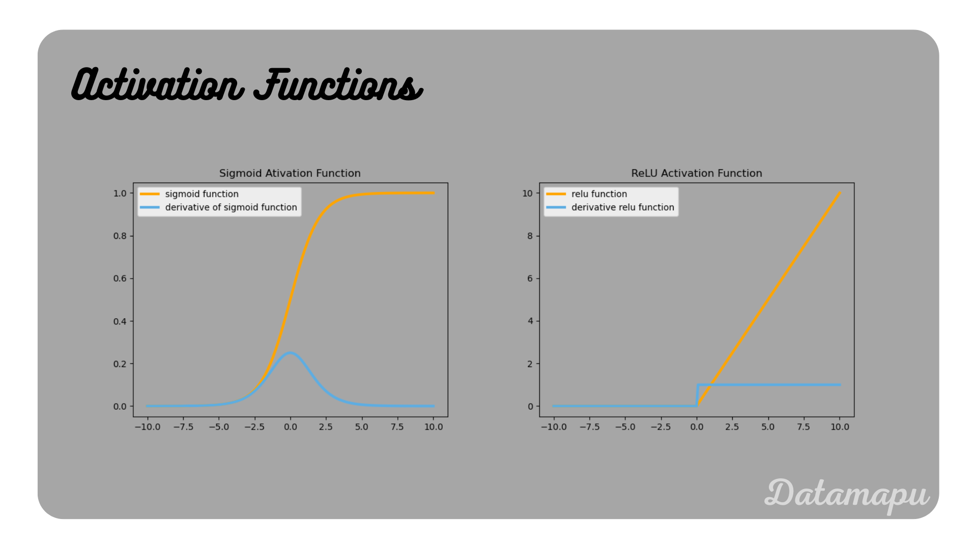
where $\hat{y}$ are the predicted values, $y$ the true values, and $w_{i}$ the weights. The prediction $\hat{y}$ is calculated by a forward pass through the Neural Network. This forward pass is the combination of several neurons and at each neuron, the activation function is applied. For a more detailed introduction to Neural Networks and their concepts, please refer to Introduction to Deep Learning. One reason for vanishing gradients lies in the construction of the activation functions. For example, the derivative of the Sigmoid activation function approaches zero for both positive and negative large values. A possibility to avoid this is choosing different activation functions like ReLu or a variant of it. In the next plot, both the Sigmoid and the ReLU activation functions are shown together with their derivatives to make the different behaviour of their derivatives clear. Another way to reduce the vanishing gradient problem is to use proper weight initialization. Different types of weight initialization have been developed. We will not go into further details here, for more information, please refer to this article. Also, batch normalization may help to reduce the vanishing gradient problem. In batch normalization, each data batch is normalized before each new layer. Exploding gradients may happen if initialized weights lead to some high loss, which keeps growing by multiplication. This can also be avoided by using a proper initialization.

loss_functions Illustration of the Sigmoid and the ReLU activation functions and their derivatives.

Summary

Gradient Descent is a technique to numerically approach the minimum of a given function. In the context of Machine Learning, we use Gradient Descent for training a model, e.g. a Neural Net. In this case, the gradient of the loss function is used to optimize the weights of the model. Different variants of Gradient Descent exist, in practice often the mini-batch Gradient Descent is used, where subsets (batches) of the training dataset are used to update the weights. This is less computationally expensive than the classical variant of (Batch-)Gradient Descent.

If this blog is useful for you, please consider supporting.