Loss Functions in Machine Learning

February 4, 2024 - 11 minutes read - 2160 words

Introduction

In Machine Learning loss functions are used to evaluate the model. They compare the true target values with the predicted ones and are directly related to the error of the predictions. During the training of a model, the loss function is aimed to be optimized to minimize the error of the predictions. It is a general convention to define a loss function such that it is minimized rather than maximized. The specific choice of a loss function depends on the problem we want to solve, e.g. whether a regression or a classification task is considered. In this article, we will discuss the most common ones, which work very well for a lot of tasks. We can, however, also create custom loss functions adapted for specific problems. Custom loss functions help to focus on the specific errors we aim to minimize. We will look at examples of custom loss functions later in this post.

loss_function

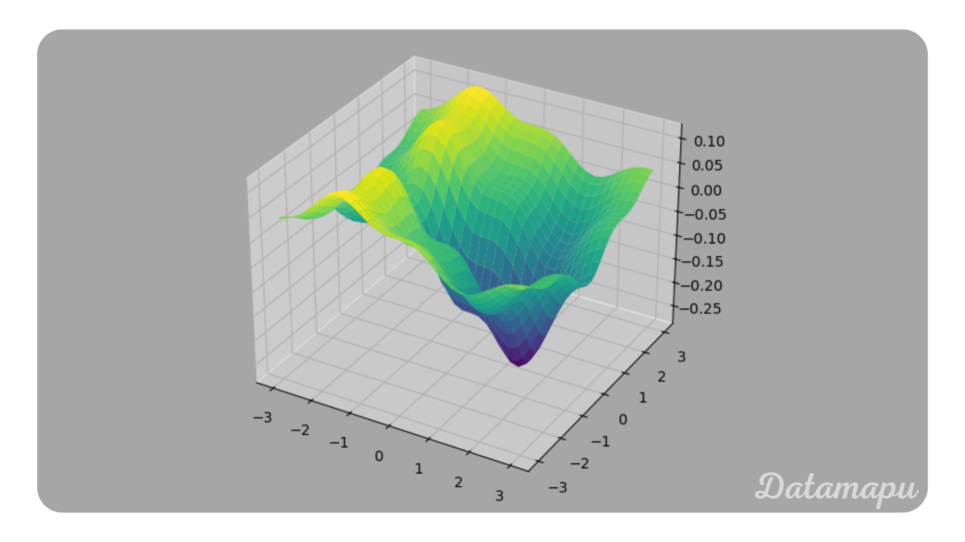
Terminology

The term Loss Function is most commonly used, however, sometimes it is also called Error Function. The outcome of the loss function is called Loss. The loss function is applied to each sample of the dataset, it is related to the Cost Function (sometimes also called Objective Function), which is the average of all loss function values. The cost function is therefore a measure of how the model performs on the entire dataset, while the loss function evaluates the loss for each sample. In practice, however, the terms Loss Function and Cost Function are often used interchangeably.

How are Loss Functions used in Machine Learning?

Loss functions can be used in different ways for training and evaluating a Machine Learning model. All Machine Learning models need to be evaluated with a metric to check how well the predictions fit the true values. These metrics can be considered as cost functions because they measure the performance of the entire dataset. Examples of such evaluation metrics are e.g. the Mean Squared Error for a regression task or the Accuracy for a classification task. More examples of common metrics can be found in the separate articles Metrics for Classification Problems and Metrics for Regression Problems. These metrics, however, are not necessarily based on the same loss function that is used during the training of a model. Depending on the underlying algorithm loss functions are used in different ways.

For Decision Trees, loss functions are used to guide the construction of the tree. For classification usually the Gini-Impurity or Entropy is used as loss function and for regression tasks the Sum of Squared Errors. These losses are minimized at each split of the tree. We can therefore say, that in a Decision Tree at each split the local minimum of the loss function is calculated. Decision Trees follow a so-called greedy search and assume that the sequence of locally optimal solutions leads to a globally optimal solution. In other words, they assume by choosing the lowest loss (error) at each split, the overall loss (error) of the model is also minimized. This assumption, however, does not always hold.

Other Machine Learning models, like e.g. Gradient Boosting or Neural Networks, use a global loss function to optimize results. The loss functions depend on the model’s parameters because the predictions are calculated based on these parameters. In a Neural Network, these parameters are the weights and the biases. During the training of such models, we aim to change these parameters such that the loss (error) between the true values and the predicted values is minimized. That is we aim to minimize the loss function. This is an iterative process. To approximate the minimum of a function numerically different optimization techniques exist. The most popular one is Gradient Descent or a variant of it. The main idea is to use the negative of the gradient of a function at a specific point to find the direction of the steepest descent to move into the direction of the minimum. That is why for such types of models, the loss function needs to be differentiable. Small steps in the direction of the minimum are taken in each training step. The parameters of the model are then updated using the gradient of the loss function. The process is illustrated in the following plot. For a more detailed explanation, please refer to the separate article about Gradient Descent.

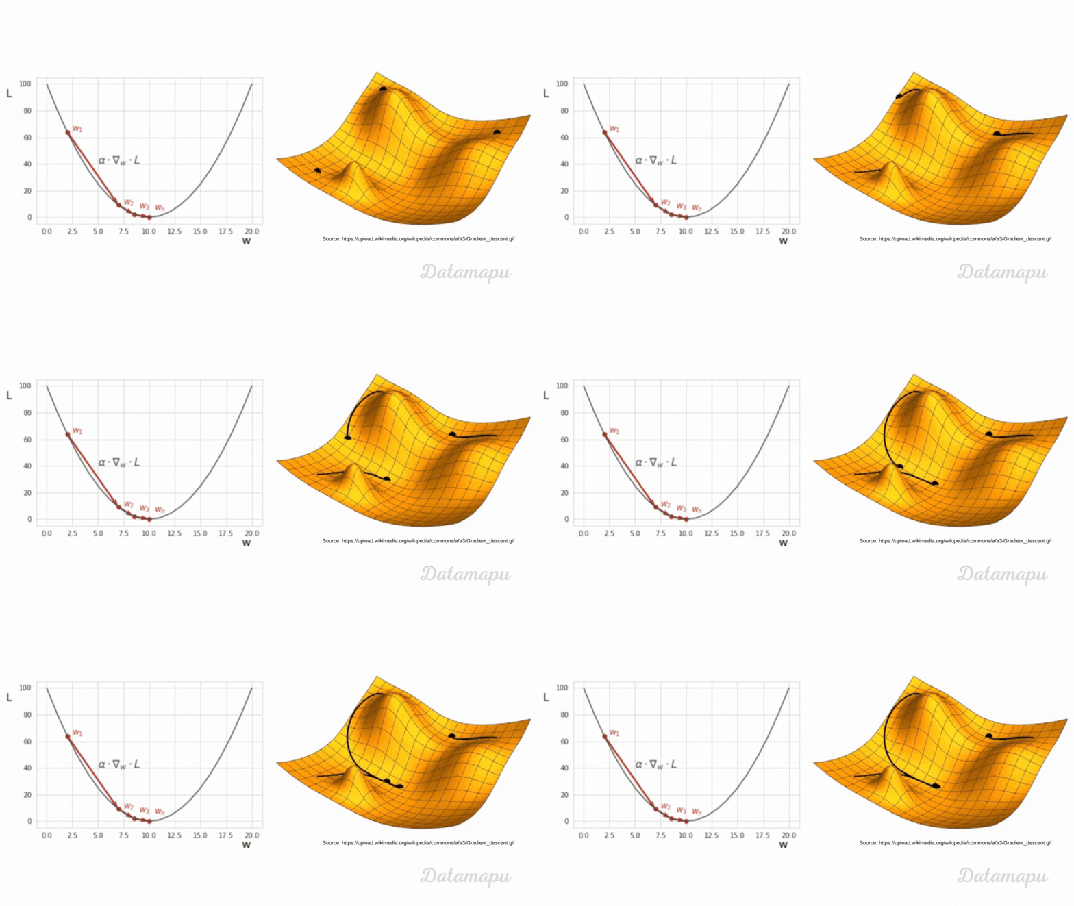ai_ml_dl Ilustration of Gradient Descent.

During the training process, the loss is calculated after each training step. If the loss decreases, we know that the model is improving, while when it increases we know that is not. The loss thus guides the model in the correct direction. Note, in contrast to Decision Trees the Loss is not calculated locally for a specific region, but globally.

Examples

The choice of the loss function used depends on the problem we are considering. Especially, we can divide them into two types. Loss functions for regression tasks and loss functions for classification tasks. In a regression task, we aim to predict continuous values as closely as possible (e.g. a price), while in a classification task, we aim to predict the probability of a category (e.g. a grade). In the following, we will discuss the most commonly used loss functions for each case, and also define a customized loss function.

Loss Functions for Regression Tasks

Mean Absolute Error

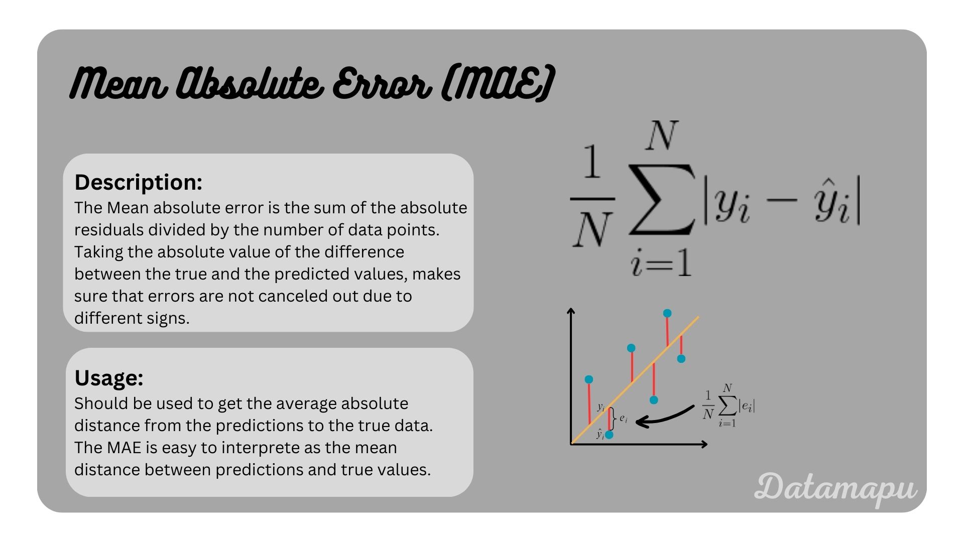
The Mean Absolute Error (MAE) or also called L1-Loss, is defined as

$$L(y_i, \hat{y}_i) = |y_i - \hat{y}_i|,$$

and accordingly the cost function over all samples

$$f(y, \hat{y}) = \frac{1}{N} \sum_{i=1}^N |y_i - \hat{y}_i|,$$

with $N$ the number of data samples, $y_i = (y_1, y_2, \dots, y_n)$ the true observation values, and $\hat{y}_i = (\hat{y}_1, \hat{y}_2, \dots, \hat{y}_N)$ the predicted values. The MAE is summarized in the following plot.

msa

Mean Squared Error

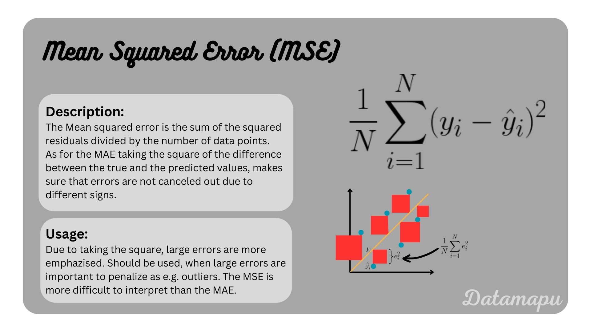
The Mean Squared Error (MSE) or also called L2-Loss, is defined as

$$L(y_i, \hat{y}_i) = (y_i - \hat{y}_i)^2,$$

and accordingly the cost function over all samples

$$f(y, \hat{y}) = \frac{1}{N} \sum_{i=1}^N (y_i - \hat{y}_i)^2,$$

mse

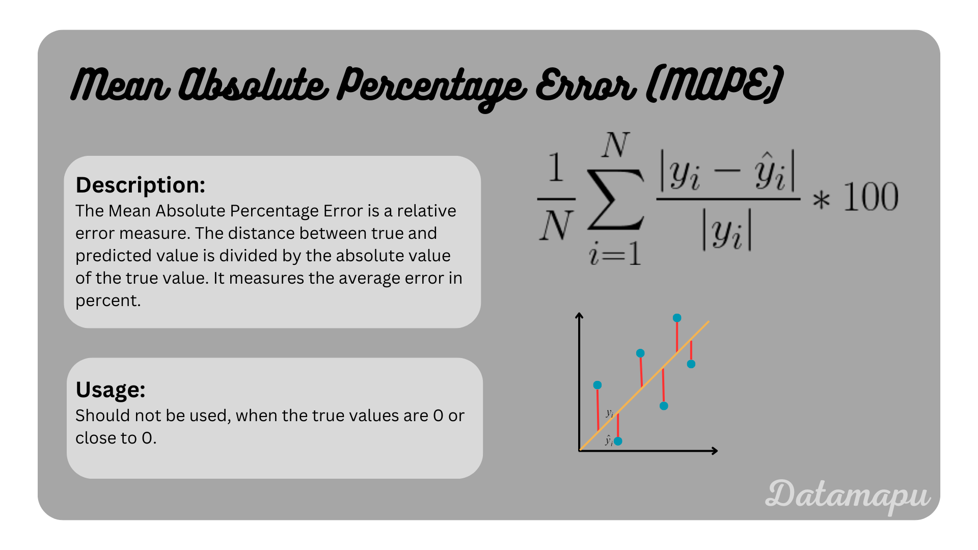
Mean Absolute Percentage Error

The Mean Absolute Percentage Error (MAPE), is defined as

$$L(y, \hat{y}) = \frac{|y_i - \hat{y}_i|}{|y_i|} \cdot 100,$$

and accordingly the cost function over all data samples

$$f(y, \hat{y}) = \frac{1}{N} \sum_{i=1}^N \frac{|y_i - \hat{y}_i|}{|y_i|} \cdot 100,$$

mse

Huber Loss

The Huber Loss is a possibility to combine the advantages of both the MSE and MAE. It is defined as

huber_loss

with $\delta$ a hyperparameter, that specifies from which point the loss should follow a linear curve instead of a quadratic curve. The Huber Loss is summarized and illustrated for different parameters in the following plot.

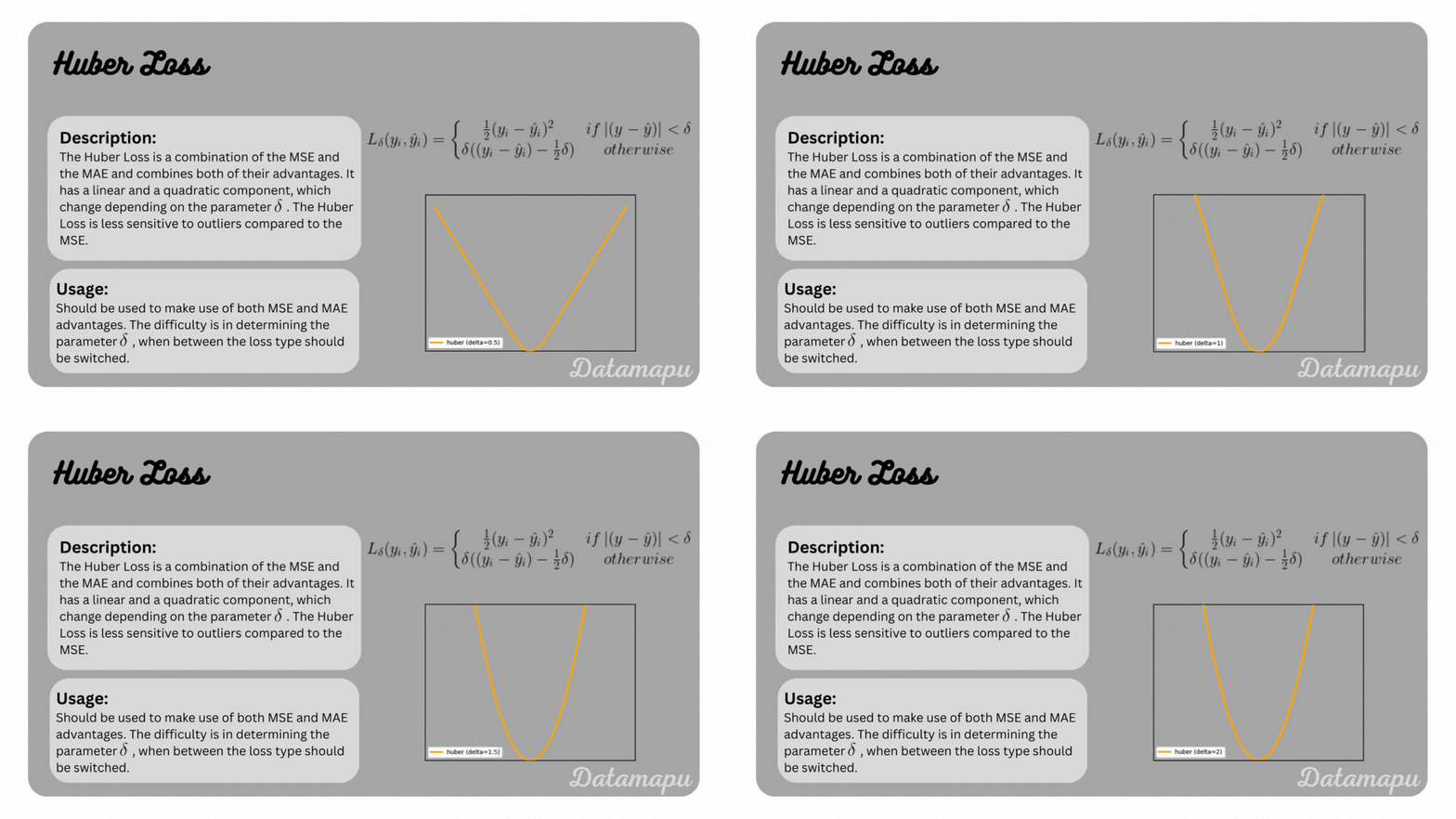huber_loss The Huber Loss.

Log-Cosh-Loss

The Log-Cosh-Loss is very similar to the Huber loss. It also combines the advantages of both MSE and MAE. From the formula, this is not as obvious as for the Huber loss, but it can be shown, that the Logcosh approximates a quadratic function when the independent variable goes to zero and a linear function when it goes to infinity [1].

$$L(y, \hat{y}) = \sum_{i=1}^N \log (\cosh (\hat{y}_i - y_i))$$

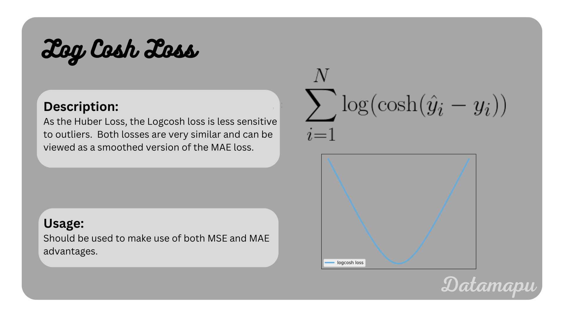logcosh_loss The Logcosh Loss.

There are of course much more loss functions for regression tasks, the ones listed above are just a selection. They are compared in the below plot.

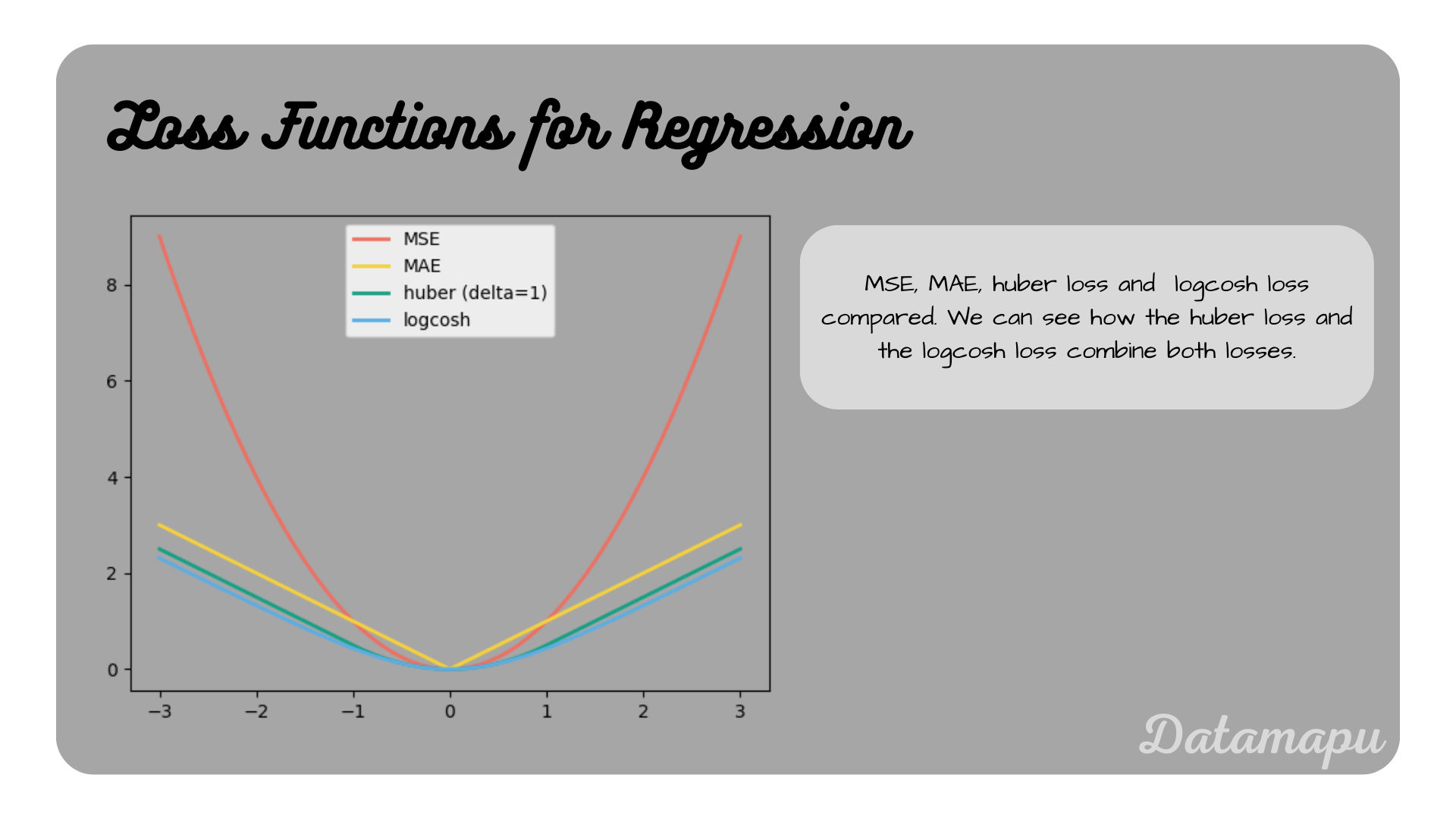loss_regression Ilustration of different loss functions for regression tasks.

Loss Functions for Classification Tasks

As for regression tasks, in classification, we use loss functions to measure the error our model makes. The difference however is, that in this case, we don’t have continuous target values, but categorical classes and the predictions of our model are probabilities.

(Binary-)Cross Entropy

(Binary-)Cross Entropy is the most used loss for classification problems. To explain Cross Entropy, we start with the special case of having two classes, i.e. a binary classification. The Cross Entropy then turns into Binary Cross Entropy (BCE), which is also often called Log Loss.

The mathematical formulation of the Cost Function is as follows

$$L(y, \hat{y}) = -\frac{1}{N}\sum_{i=1}^N{\Big(y_i\log(\hat{y}_i) + (1 - y_i)\log(1 - \hat{y}_i)\Big)},$$

with $y = (y_1, \dots, y_N)$ the true label ($0$ or $1$) and $\hat{y} = (\hat{y}_1, \dots, \hat{y}_N)$ the predicted probability. To understand how Binary Cross Entropy works, let’s consider just one sample. That means we can forget the outer sum over $i$ and get the loss function

$$L(y_i, \hat{y}_i) = -y_i\log(\hat{y}_i) - (1 - y_i)\log(1 - \hat{y}_i).$$

Let’s consider two possible target outcomes. For the case $y_i = 0$, the first part of the sum vanishes and only

$$L(y_i, \hat{y}_i) = - \log(1-\hat{y}_i)$$

remains. On the other hand, for the case $y_i = 1$, the second part of the sum vanishes and only

$$L(y_i, \hat{y}_i) = - \log(\hat{y}_i)$$

remains. These two functions are shown in the following plot.

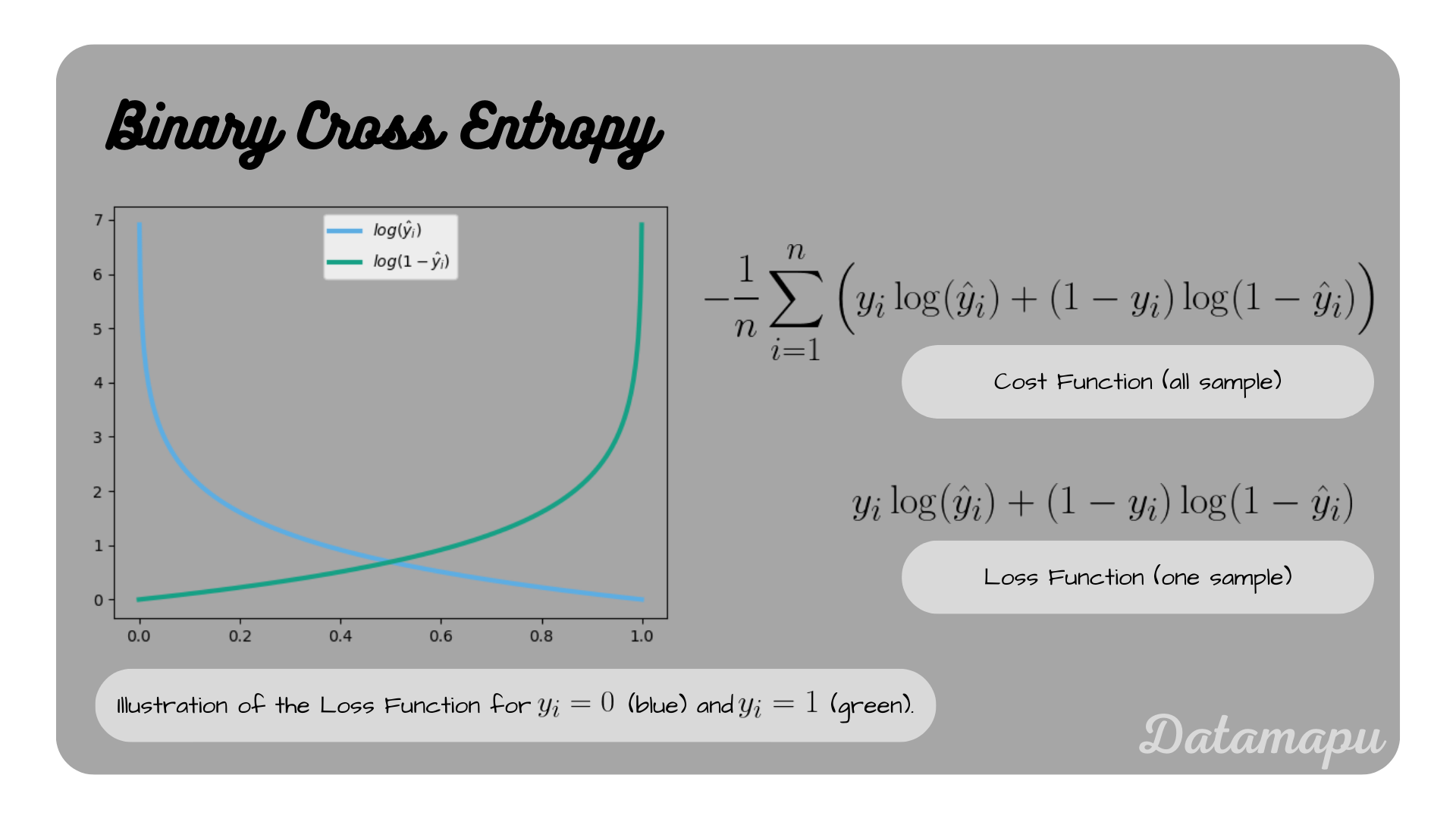logcosh_loss The Binary Cross Entropy Loss.

We know that $\hat{y}_i$ is a probability and thus can only take values between $0$ and $1$. We can see that for the case $y_i = 0$ the loss is close to $0$, when $\hat{y}_i$ is close to $0$ and it increases if $\hat{y}_i$ approaches $1$. That means the Binary Cross Entropy penalizes more the further away the predicted probability is from the true value. The same holds if $y_i = 1$. In this case, the loss is high if $\hat{y}_i$ is close to $0$ and low if it approaches $1$.

The more general formulation for $M>2$ classes of the Cross Entropy is

$$L(y, \hat{y}) = -\frac{1}{N}\sum_{j=1}^M\sum_{i=1}^N{y_{i,j}\log(\hat{y}_{i,j})}.$$

Hinge Loss

The Hinge Loss is especially used by Support Vector Machines (SVM). SVM is a type of Machine Learning model, which aims to create hyperplanes (or in two dimensions decision boundaries), which can be used to separate the data points into classes. The Hinge Loss is used to measure the distance of points to the hyperplane or decision boundary. For binary classification, it is defined as

$$L(y_i, \hat{y}_i) = max(0, 1 - y_i \cdot \hat{y}_i),$$

with $\hat{y}_i$ the predicted value and $y_i$ the true target value for $i = 1, 2, \dots N$. The convention is that the true values have values $-1$ and $1$. The Hinge Loss is zero, when $y_i\cdot\hat{y}_i >= 1$, which is the case for $y_i = 1$ and $\hat{y}_i >= 1$ or $y_i = -1$ and $\hat{y}_i <= -1$. In both cases, the data point was correctly classified, thus the loss of $0$ means we are not penalizing our model. For the cases $y_i = 1$ and $\hat{y}_i < 1$ and $y_i = -1$ and $\hat{y}_i > -1$, $y_i \cdot \hat{y}_i < 1$ and the Loss is therefore positive. The further away $\hat{y}_i$ is from the true value the more increases the loss.

The Hinge Loss can be extended to multi-class classification. This is, however, not in the scope of this article. An explanation can be found on Wikipedia.

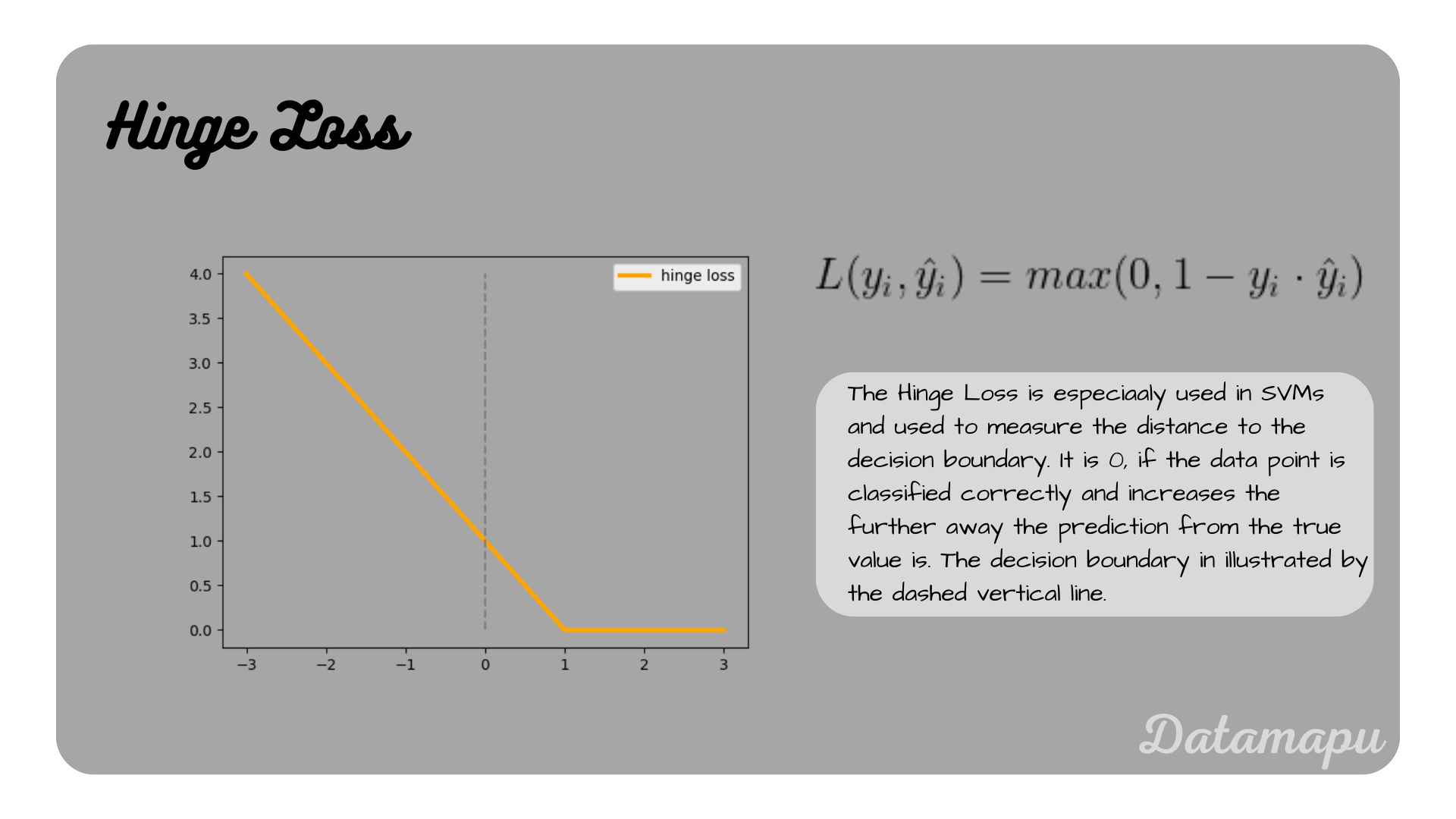hinge_loss The Hinge Loss illustrated.

Example for a custom Loss Function

The above discussed examples are the most common ones, however, we can define a Loss Function specific to our needs. We learned that the MSE penalizes outliers more than the MAE. If we want our Loss to penalize even stronger the outliers, we could for example define loss of degree $4$ as follows

$$L(y_i, \hat{y}_i) = (y_i - \hat{y}_i)^4.$$

We can also define an assymentric Loss that penalizes more negative values than positive values

asym_loss

in both cases with $\hat{y} = (y_1, \dots, y_N)$ the predicted value and $y = (y_1, \dots, y_N)$ the true values. Customized loss functions may help our model to learn. These were two examples for regression tasks, custom loss functions can however also be created for classification tasks.

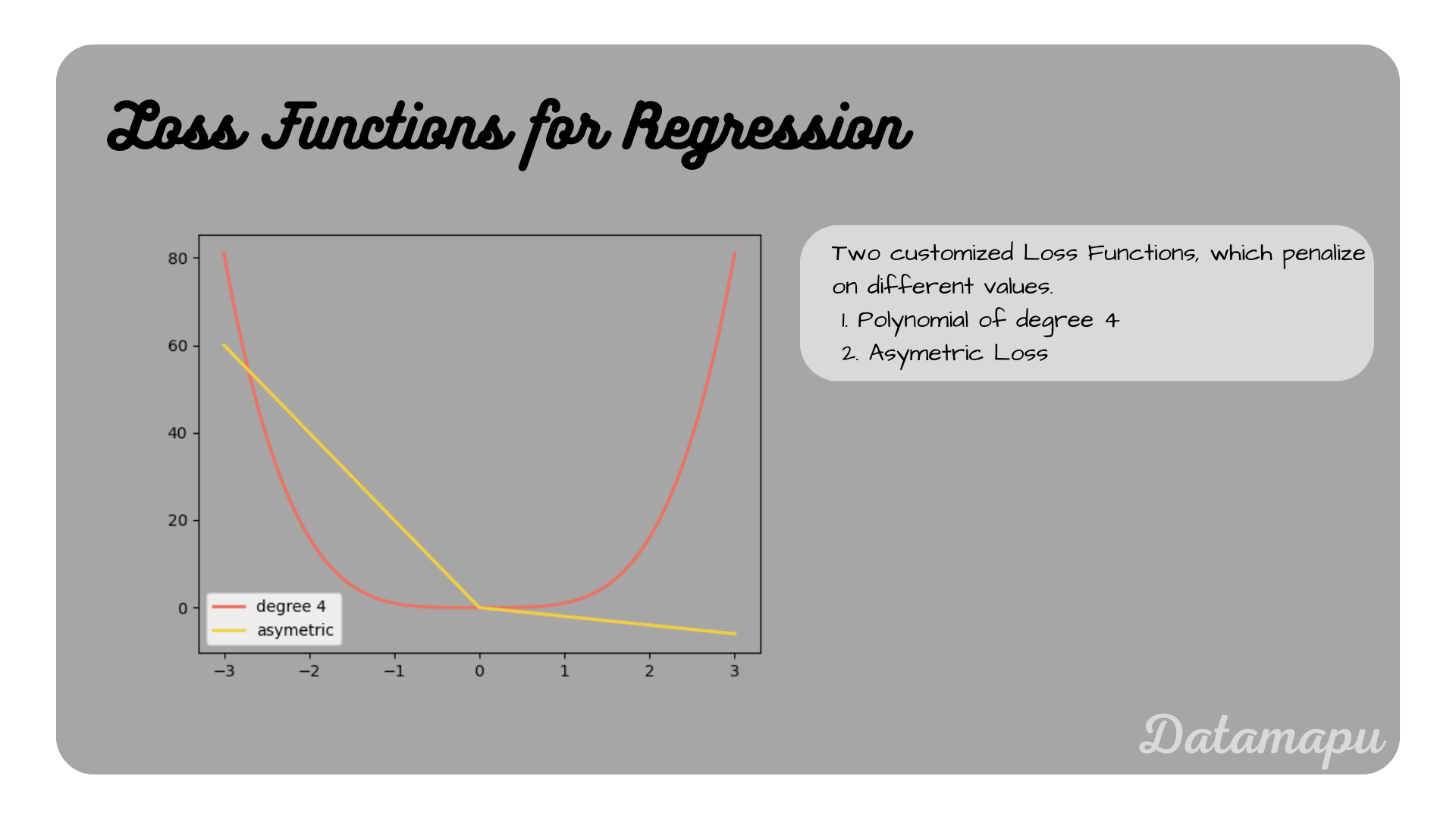custom_loss Two examples of custom Loss Functions.

Specific Machine Learning Models and their Loss Functions

Some Machine Learning algorithms have a fixed loss function, while others are flexible and the loss function can be adapted to the specific task. The following table gives a (non-exhaustive) overview of some popular Machine Learning algorithms and their corresponding loss functions. Important to keep in mind is that the loss function needs to be differentiable if some form of Gradient Descent is performed, e.g. in Neural Networks or Gradient Boosting.

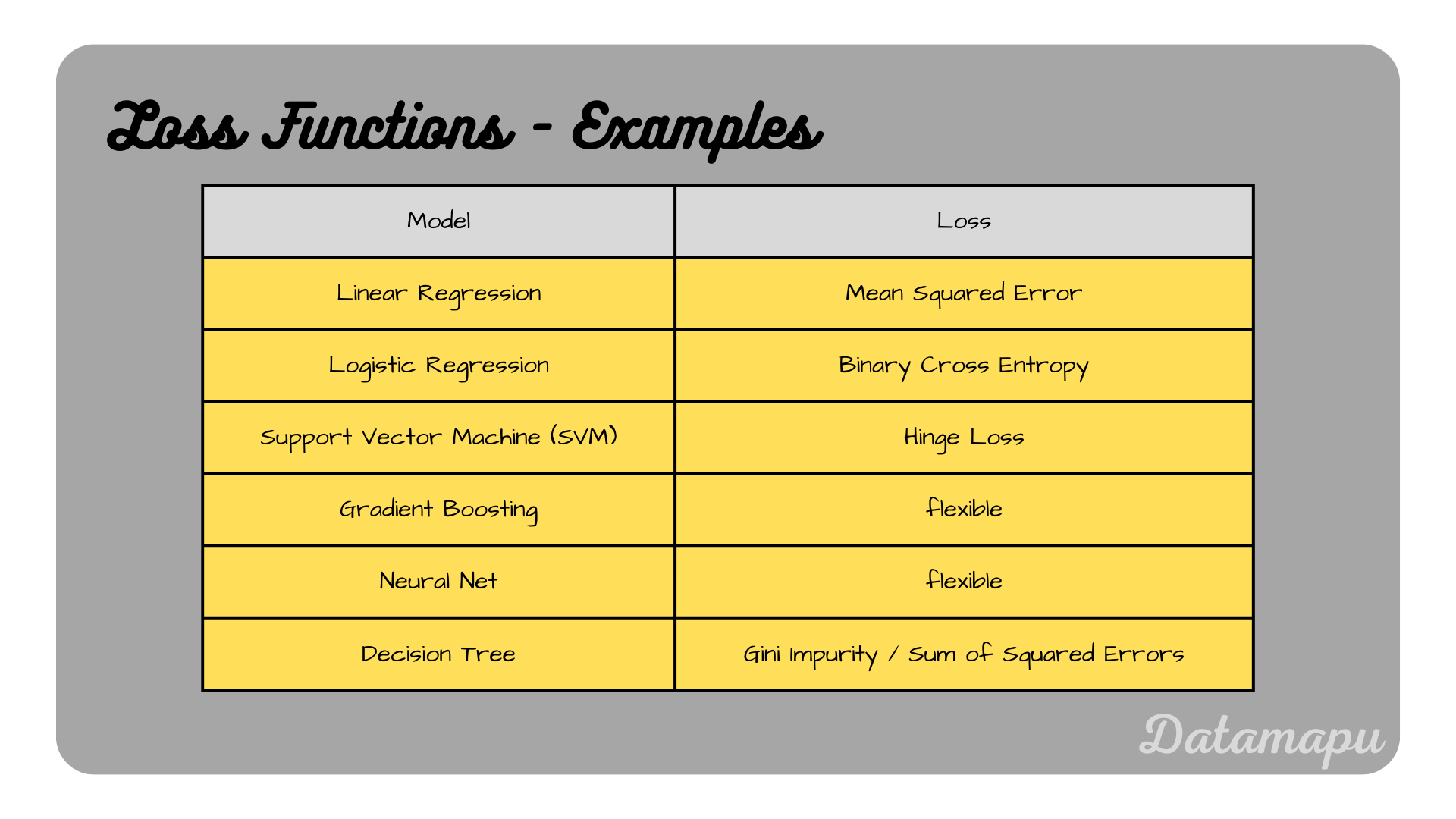loss_functions_examples Examples for Machine Learning models and their Loss Functions.

Summary

Loss functions are used to evaluate a model and to analyze if it is learning. We discussed typical loss functions for regression and classification tasks and also saw two examples of customized loss functions. Choosing an appropriate loss function is very important because it is used to evaluate and improve the model performance. It should thus reflect well the metric that is important for the project so that errors are minimized accordingly.