Gradient Boost for Classification - Explained

April 14, 2024 - 12 minutes read - 2385 words

Introduction

Gradient Boosting is an ensemble machine learning model, that - as the name suggests - is based on boosting. An ensemble model based on boosting refers to a model that sequentially builds models, and the new model depends on the previous model. In Gradient Boosting these models are built such that they improve the error of the previous model. These individual models are so-called weak learners, which means they have low predictive skills. The ensemble of these weak learners builds the final model, which is a strong learner with a high predictive skill. In this post, we go through the algorithm of Gradient Boosting in general and then concretize the individual steps for a classification task using Decision Trees as weak learners and the log-loss function. There will be some overlapping with the article Gradient Boosting for Regression - Explained, where a detailed explanation of Gradient Boosting is given, which is then applied to a regression problem. However, in this article, do not go into the details of the general formulation, for that please refer to the previously mentioned post. If you are interested in a concrete example with detailed calculations, please refer to Gradient Boosting for Regression - Example for a regression problem and Gradient Boosting for Classification - Example for a classification problem.

The Algorithm

Gradient Boosting is a boosting algorithm that aims to build a series of weak learners, which together act as a strong learner. In Gradient Boosting the objective is to improve the error of the preceeding model by minimizing its loss function using Gradient Descent. That means the weak learners are built up on the error and not up on the targets themselves as in other boosting algorithms like AdaBoost.

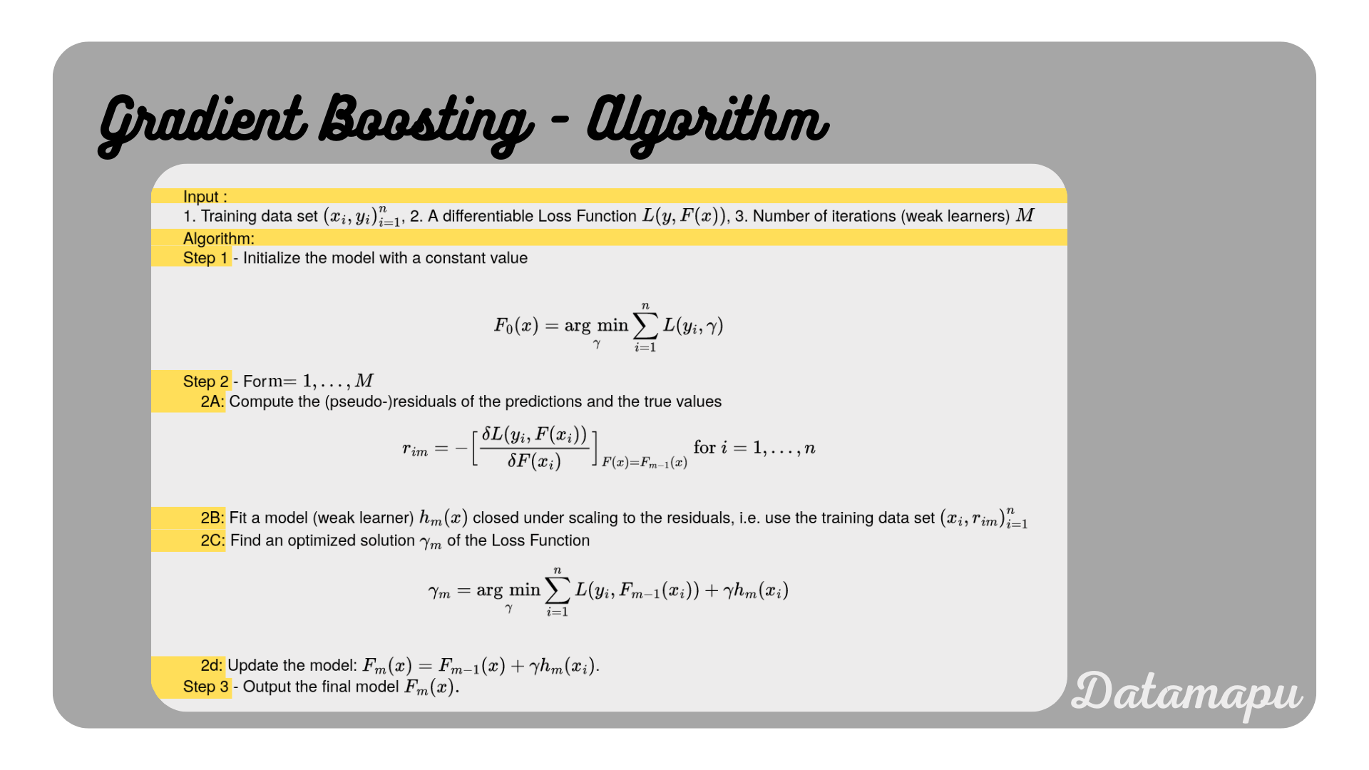
In the following, the algorithm is described for the general case. The notation is adapted from Wikipedia. The general case is explained in Gradient Boosting for Regression - Explained, in this post, we apply them to the special case of a binary classification using Decision Trees as weak learners and the log-loss as a loss function.

“gradient boosting algorithm” Gradient Boosting Algorithm. Adapted from Wikipedia.

Let’s look at the individual steps, for the special case of a binary classification. As loss function, we use the log-loss, which is defined as

$$L\big(y_i, p_i\big) = - y_i\cdot \log p_i - (1 - y_i)\cdot \log\big(1 - p_i\big),$$

with $y_i$ the true values and $p_i$ the predicted propabilities. To ensure that $p_i$ represent probabilities, we use the sigmoid function to convert the model output to values between $0$ and $1$, i.e. $p_i = \sigma\big(F_{m-1}(x_i)\big)$. With that, we can rewrite the loss function, depending on the model output

$$L\big(y_i, \gamma\big) = - y_i\cdot \log\big(\sigma(\gamma)\big) - (1 - y_i)\cdot \log\big(1 - \sigma(\gamma)\big),$$

with $\gamma$ the predicted values and $p = \sigma(\gamma) = \frac{1}{1 + e^{-\gamma}}$.

Let ${(x_i, y_i)}_{i=1}^n = {(x_1, y_1), \dots, (x_n, y_n)}$ be the training data, with $x = x_0, \dots, x_n$ the input features and $y = y_0, \dots, y_n$ the target values, the algorithm is then as follows.

Step 1 - Initialize the model with a constant value

The first initialization of the model is given by

$$F_0(x) = \underset{\gamma}{\text{argmin}}\sum_{i=1}^n L(y_i, \gamma). $$

Using the log-loss as formulated above, this turns into

$$F_0(x) = \underset{\gamma}{\text{argmin}}\sum_{i=1}^n \big(- y_i\cdot \log\big(\sigma(\gamma)\big) - (1 - y_i)\cdot \log\big(1 - \sigma(\gamma)\big)\big), $$

The expression $\underset{\gamma}{\textit{argmin}}$ refers to finding the value $\gamma$ which minimizes the equation. To find a minimum, we need to set the derivative equal to $0$. Let’s calculate the derivative with respect to $\gamma$.

$$\frac{\delta}{\delta \gamma} \sum_{i=1}^n L = \frac{\delta}{\delta \gamma}\sum_{i=1}^n\Big( - y_i\cdot \log\big(\sigma(\gamma)\big) - (1 - y_i)\cdot \log\big(1 - \sigma(\gamma)\big) \Big).$$

To calculate this derivative, we need to use the chain rule and we need to remember the derivative of the logarithm, which is.

$$\frac{d}{dz} \log(z) = \frac{1}{z}$$

together with the chain rule

$$\frac{d}{dz} \log(f(z)) = \frac{1}{f(z)} f’(z).$$

Note, that this is the derivative of the natural logarithm. If the logarithm is to a different base the derivative changes. Further, we need the derivative of the sigmoid function, which is

$$\sigma\prime(z) = \sigma(z)\cdot(1 - \sigma(z)).$$

The derivation of this equation can be found here.

With this we get

$$\frac{\delta}{\delta \gamma} \sum_{i=1}^n L = \sum_{i=1}^n\Big(- y_i \frac{1}{\sigma(\gamma)}\sigma(\gamma)\big(1 - \sigma(\gamma)\big) - (1 - y_i)\frac{1}{1 - \sigma(\gamma)}\big(-\sigma(\gamma)(1 - \sigma(\gamma) \big)\Big).$$

This can be simplified to

$$\frac{\delta}{\delta \gamma} \sum_{i=1}^n L = \sum_{i=1}^n\Big(- y_i(1 - \sigma(\gamma)) + (1 - y_i) \sigma(\gamma)\Big)$$ $$\frac{\delta}{\delta \gamma} \sum_{i=1}^n L = \sum_{i=1}^n\Big(- y_i + y_i \sigma(\gamma) + \sigma(\gamma) - y_i \sigma(\gamma)\Big)$$ $$\frac{\delta}{\delta \gamma} \sum_{i=1}^n L = \sum_{i=1}^n\Big(\sigma(\gamma) - y_i\Big).$$

Now we set the derivative to $0$ to find the minimum

$$0 = \sum_{i=1}^n\Big(\sigma(\gamma) - y_i\Big).$$

This can be transformed to

$$\sum_{i=1}^n\sigma(\gamma) = \sum_{i=1}^n y_i.$$

$$n\sigma(\gamma) = \sum_{i=1}^n y_i.$$

$$\sigma(\gamma) = \frac{1}{n}\sum_{i=1}^n y_i.$$

The right-hand side of this equation corresponds to the probability of the positive class $p = \frac{1}{n}\sum_{i=1}^n y_i$. Using $\sigma(\gamma) = \frac{1}{1 + e^{-\gamma}}$, we get

$$p = \frac{1}{1 + e^{-\gamma}}$$ $$\frac{1}{p} = 1 + e^{-\gamma}$$ $$e^{-\gamma} = \frac{1}{p} - 1.$$

Applying the logarithm this leads to

$$-\gamma = \log\Big(\frac{1}{p} - 1\Big)$$ $$-\gamma = \log\Big(\frac{1-p}{p}\Big).$$

Using logarithmic transformations we get

$$\gamma = \log\Big(\frac{p}{1-p}\Big).$$

The last transformation is explained in more detail in the appendix.

This expression refers to the log of the odds of the target variable, which is used to initialize the model for the specific case of a binary classification.

The next step is performed $M$ times, where $M$ refers to the number of weak learners used.

Step 2 - for $m = 1$ to $M$

2A. Compute (pseudo-)residuals of the predictions and the true values.

The (pseudo-) residuals are defined as pseudo_residual

for $i = 1, \dots, n$.

That is we need to calculate the derivative of the loss function with respect to the predictions.

With the loss function $L(y_i, p_i)$ defined above, where $p$ are the probabilities after applying the sigmoid function, $p_i= \sigma\big(F_{m-1}(x_i)\big) = \sigma(y_i)$, this turns into

$$r_{im} = -\frac{\delta L(y_i, p_i)}{\delta \gamma}.$$

To calculate this derivative we need to use the chain-rule

$$\frac{\delta L}{\delta \gamma} = \frac{\delta L}{\delta p_i}\frac{\delta p_i}{\delta \gamma}.$$

We calculate the first derivative $\frac{\delta L}{\delta p_i}$.

$$\frac{\delta L}{\delta p_i} = \frac{\delta\Big(-y_i\cdot \log p_i - (1 - y_i)\cdot \log(1 - p_i)\Big)}{\delta p_i},$$ $$\frac{\delta L}{\delta p_i} = \frac{-y_i\cdot\delta \log p_i}{\delta p_i} - \frac{(1 - y_i)\cdot\delta \log\big(1 - p_i\big)}{\delta p_i}$$

Using the derivative of the logarithm as above, this leads to

$$\frac{\delta L}{\delta p_i} = - \frac{y_i}{p_i} + \frac{1 - y_i}{1 - p_i}$$

For the second part of the derivative we again need the derivative of the sigmoid function.

$$\frac{\delta p_i}{\delta \gamma} = \frac{\delta \sigma (\gamma)}{\delta \gamma} = \sigma (\gamma) \cdot \big(1 - \sigma (\gamma)\big) = p_i\cdot(1-p_i)$$

Now, we can calculate the derivative $\frac{\delta L}{\delta \gamma}$ as

$$\frac{\delta L}{\delta \gamma} = -\Big(\frac{y_i}{p_i} - \frac{1 - y_i}{1 - p_i}\Big)\cdot p_i \cdot (1 - p_i)$$ $$\frac{\delta L}{\delta \gamma} = -\big(y_i (1 - p_i) - (1 - y_i) p_i\big)$$ $$\frac{\delta L}{\delta \gamma} = p_i - y_i$$

That is the (pseudo-)residuals are given as

$$r_{im} = - (p_i^{m-1} - y_i^{m-1}),$$ $$r_{im} = y_i^{m-1} - p_i^{m-1}$$

with $y_i^{m-1}$ the output of the previous weak learner and $p_i^{m-1}$ the corresponding probabilities.

2B. Fit a model (weak learner) closed after scaling $h_m(x)$.

In this step, we fit a weak model to the input features and the residuals $(x_i, r_{im})_{i=1}^n$. The weak model in our special case is a Decision Tree for classification, which is pruned by the number of trees or leaves.

2C. Find an optimized solution $\gamma_m$ for the loss function.

In this step the optimization problem

$$\gamma_m = \underset{\gamma}{\text{argmin}}\sum_{i=1}^nL(y_i, F_{m-1}(x_i) + \gamma h_m(x_i)), (2a)$$

where $h_m(x_i)$ is the just fitted model (weak learner) at $x_i$ needs to be solved. The derivation for the special case of Decision Trees can be rewritten as

$$h(x_i) = \sum_{j=1}^{J_m} b_{jm} 1_{R_{jm}}(x), (2b)$$

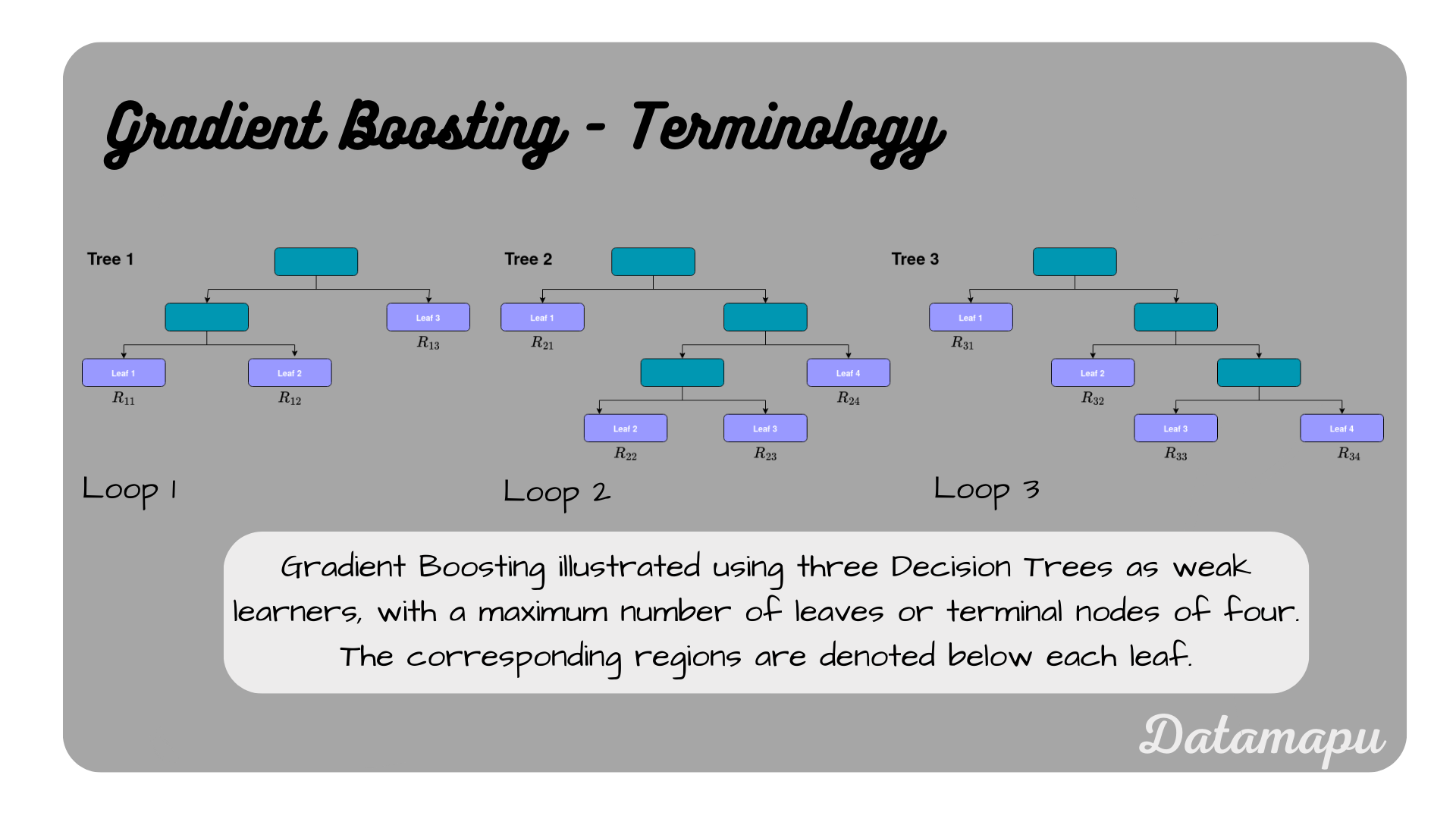
where $J_m$ is the number of leaves or terminal nodes of the tree, and $R_{1m}, \dots R_{J_{m}m}$ are so-called regions. The regions refer to the terminal nodes of the Decision Tree. We use a pruned Decision Tree, that is the terminal nodes will very likely contain several different samples. The prediction for each region $j$ is denoted as $b_{jm}$ in the above equation. We will look at how these predictions are determined in a bit. The formulation is illustrated in the following plot, which should make the concept of the regions clearer.

Gradient Boosting Terminology Terminology for Gradient Boosting with Decision Trees.

Now, let’s consider the predictions $b_{jm}$ of each region $j$. In a regression problem, the final prediction is determined as the mean of the individual samples in each leaf (region). For a classification problem, this is a bit different. One possibility would be to use the majority class, that is the class that appears mostly in each leaf. However, for Gradient Boosting usually, a different method is chosen, which is the weighted average of the samples in each leaf (region). In this case, in which we predict the residuals, this is defined as

$b_{jm} =\frac{\sum_{i\in R_{jm}} r_{im}}{|R_{jm}|}, (2c)$

with $|R_{jm}|$ the number of samples in $R_{jm}$, and $r_{im}$ the residual for sample $i$.

Coming back to equation (2a), we aim to find $\gamma_m$ that minimizes the loss function. As explained in Wikipedia [1] and Friedman (1999) [2] for a Decision Tree as an underlying model, this step is a bit modified. Individual optimal values $\gamma_{jm}$ for each region $j$ are chosen, instead of a single $\gamma_{m}$ for the whole tree. The coefficients $b_{jm}$ can then be discarded and equation (2a) can be rewritten as

$$\gamma_{jm} = \underset{\gamma}{\text{argmin}}\sum_{x_i \in R_{jm}} L(y_i, F_{m-1}(x_i) + \gamma).$$

Note, that the summation is only over the elements of the region. Using the log-loss $L\big(y_i, p\big) = - y_i\cdot \log p - (1 - y_i)\cdot \log\big(1 - p\big)$, equation (2a) converts into

$$\gamma_{jm} = \underset{\gamma}{\text{argmin}}\sum_{x_i \in R_{jm}} L\big(y_i, p_i\big) = \underset{\gamma}{\text{argmin}}\sum_{x_i \in R_{jm}} \Big(- y_i\cdot \log p_i - (1 - y_i)\cdot \log\big(1 - p_i\big)\Big),$$

with $p_i = \sigma \big(F_{m-1}(x_i)\big).$

To solve for this we would need to calculate the derivative with respect to $\gamma$ and set it to $0$. Here it becomes a bit more complex than in the case of a regression problem. We are not going into detail here, but the solution of this optimization problem is usually approximated by

$$\gamma_m \approx \frac{\sum_{i=1}^n r_{im}h_m(x_i)}{\sum_{i=1}^n |h_m(x_i)| (1 - |h_m(x_i)|}),$$

with $r_{im} = y_i - p_i^{m-1}$ the (pseudo-)residuals.

2D. Update the model.

In this step, we update our model $F_{m}$ using the previous model $F_{m-1}$ and the weak learner $h_m(x)$ fitted to the residuals developed during this loop. The general formulation

$$F_m(x) = F_{m-1}(x) + \gamma_m h_m(x)$$

can be rewritten for the special case of using Decision Trees as weak learners to

$$F_{m}(x) = F_{m-1}(x) + \alpha \sum_{j=1}^{J_m} \gamma_{jm}1(x\in R_{jm}).$$

In this equation $\alpha$ is the learning rate or step size that determines the influence of the weak learners. The learning rate $\alpha$ is a hyperparameter which is a number between 0 and 1. The choice of the learning rate is important to tackle the Bias-Variance Tradeoff. A learning rate close to $1$ usually reduces the bias but introduces a higher variance and vice versa. A lower learning rate may help to reduce overfitting.

Step 3 - Output final model $F_M(X)$.

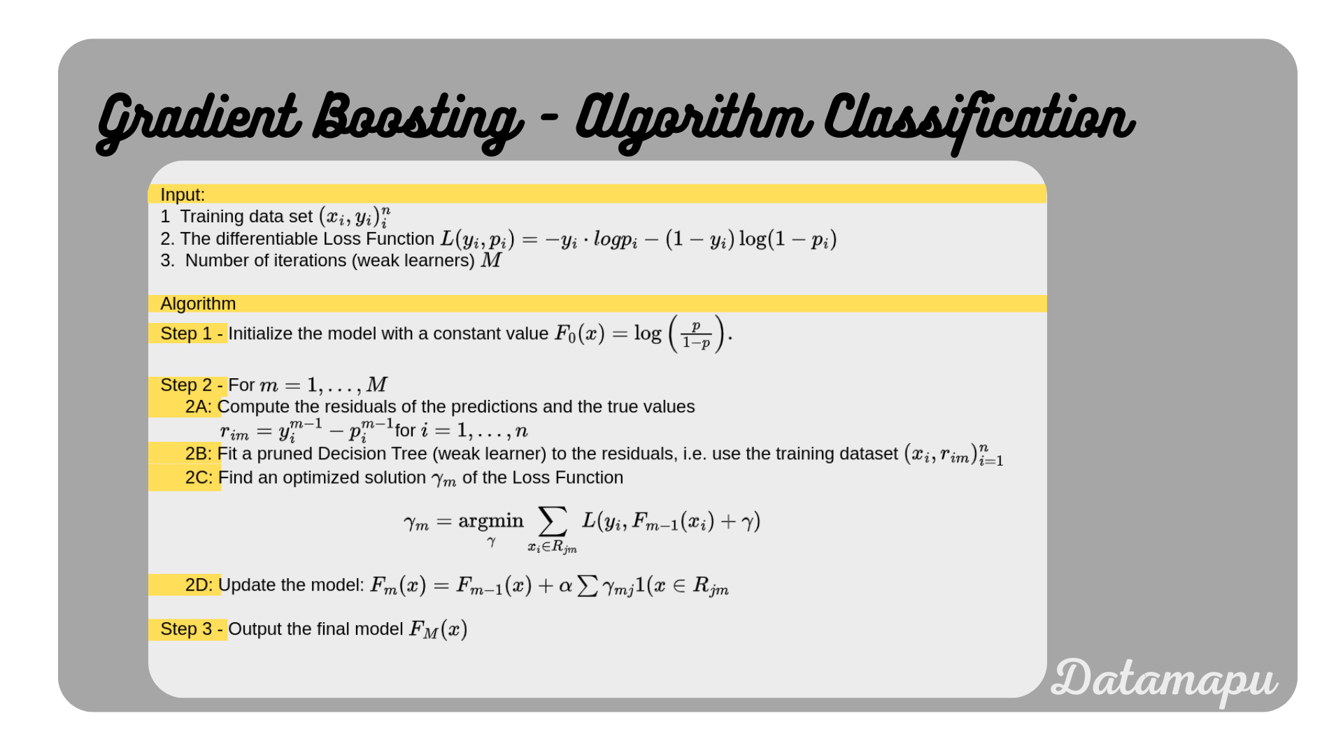
The individual steps of the algorithm for the special case of a binary classification using Decision Trees, and the above specified loss, are summarized below.

Gradient Boosting for Classification Gradient Boosting Algorithm simplified for a binary classification task.

Gradient Boosting in Python

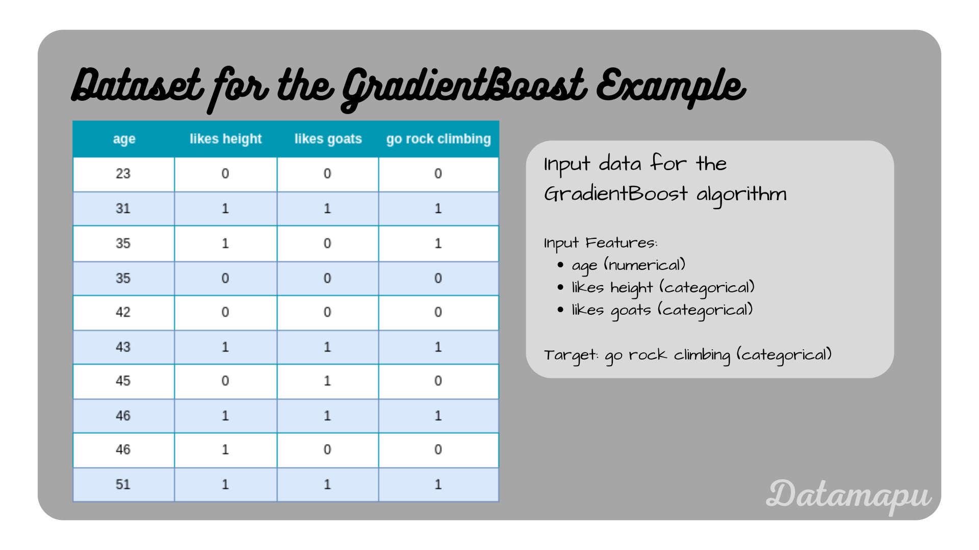
To perform gradient boosting for classification in Python, we can use sklearn. The GradientBoostingClassifer method can be used for binary and multiple classification tasks. The weak learners in sklearn are Decision Trees and cannot be changed. Let’s consider a simple dataset, consisting of 10 data samples. It is the same dataset we use in Decision Trees for Classification - Example.

gradient boosting class data Dataset considered in this example

In Python we can read this data into a pandas dataframe.

1
2
3
4
5
6
7
8
import pandas as pd

data = {'age': [23, 31, 35, 35, 42, 43, 45, 46, 46, 51], 
        'likes goats': [0, 1, 0, 0, 0, 1, 1, 1, 0, 1], 
        'likes height': [0, 1, 1, 0, 0, 1, 0, 1, 1, 1], 
        'go rock climbing': [0, 1, 1, 0, 0, 1, 0, 1, 0, 1]}

df = pd.DataFrame(data)

Now we can fit a model to the data. The GradientBoostingClassifier method from sklearn offers a set of hyperparameters that can be changed to optimize the model. For this example, we set only two hyperparameters. The first one is the number of weak learners, that is the number of Decision Trees - n_estimators. For this simple dataset, we choose $3$ weak learners. The second hyperparameter we set is max_depth, which is the maximal depth of the Decision Trees. In this example, we set it to $2$. For a complete guide of all possible hyperparameters, please refer to the documentation of sklearn.

1
2
3
4
5
6
7
8
9
from sklearn.ensemble import GradientBoostingClassifier

X = df[['age', 'likes goats', 'likes height']].values
y = df[['go rock climbing']].values.reshape(-1,)
clf = GradientBoostingClassifier(
    n_estimators=3, 
    max_depth=2
    )
clf.fit(X, y)

To make the predictions and calculate the score, which in this case is the mean accuracy of all samples, we can also use sklearn.

1
2
y_pred = clf.predict(X)
score = clf.score(X, y)

For this simplified example, we receive the predictions $[0, 1, 0, 0, 0, 1, 0, 1, 0, 1]$ and a score of $0.9$.

Summary

In this article, we discussed the Gradient Boosting algorithm for the special case of a binary classification. Gradient Boosting is a powerful ensemble learning method, which is in general based on Decision Trees. However, other weak learners are possible. In this case, the optimization of the loss function is approximated, in contrast to the Gradient Boosting for regression algorithm, where an analytical solution can be found relatively easily. In practice, sklearn can be used to develop and evaluate Gradient Boosting models in Python. For a more detailed example in Python on a larger dataset, please refer to this notebook on kaggle, which describes a regression problem. Adjusting the model and the evaluation metric the application to a classification problem is similar.

Appendix

Derive $-log\big(\frac{x}{y}\big) = log\big(\frac{y}{x}\big)$:

$$-log \big(\frac{x}{y}\big) = - \big(log(x) - log(y)\big) = log(y) - log(x) = log\big(\frac{y}{x}\big)$$