Gradient Boost for Regression - Explained

January 31, 2024 - 13 minutes read - 2758 words

Introduction

Gradient Boosting, also called Gradient Boosting Machine (GBM) is a type of supervised Machine Learning algorithm that is based on ensemble learning. It consists of a sequential series of models, each one trying to improve the errors of the previous one. It can be used for both regression and classification tasks. In this post, we introduce the algorithm and then explain it in detail for a regression task. We will look at the general formulation of the algorithm and then derive and simplify the individual steps for the most common use case, which uses Decision Trees as underlying models and a variation of the Mean Squared Error (MSE) as loss function. Please find a detailed example, where this is applied to a specific dataset in the separate article Gradient Boosting for Regression - Example. Gradient Boosting can also be applied for classification tasks. This is covered in the articles Gradient Boosting for Classification - Explained and Gradient Boosting for Classification - Example.

The Algorithm

Gradient Boosting is, as the name suggests, an ensemble model that is based on boosting. In boosting, an initial model is fit to the data. Then a second model is built on the results of the first one, trying to improve the inaccurate results of the first one, and so on until a series of additive models is built, which together are the ensemble model. The individual models are so-called weak learners, which means that they are simple models with low predictive skill. They are only a bit better than random chance. The idea is to combine a set of weak learners to achieve one strong learner, i.e. a model with high predictive skill.

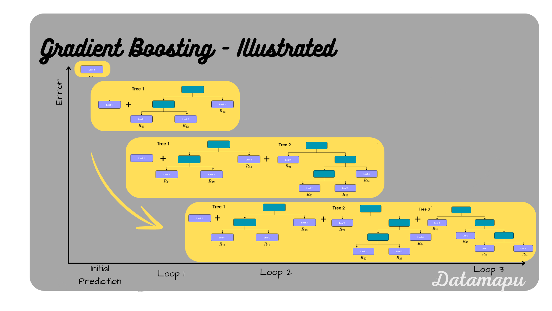Gradient Bosting illustrated Gradient Boosting illustrated.

The most popular underlying models in Gradient Boosting are Decision Trees, however using other models, is also possible. When a Decision Tree is used as a base model the algorithm is called Gradient Boosted Trees, and a shallow tree is used as a weak learner. Gradient Boosting is a supervised Machine Learning algorithm, that means we aim to find a mapping that approximates the target data as good as possible. This is done by minimizing a loss function, that measures the error between the true and the predicted values. Common choices for loss functions in the context of Gradient Boosting are a variation of the mean squared error for a regression task and the logarithmic loss for a classification task. It can however be any differentiable function.

In this section, we go through the individual steps of the algorithm in detail. The algorithm was first described by Friedman (1999)[1]. For the explanation, we will follow the notations used on Wikipedia. The next plot shows the very general formulation of Gradient Boosting following Wikipedia.

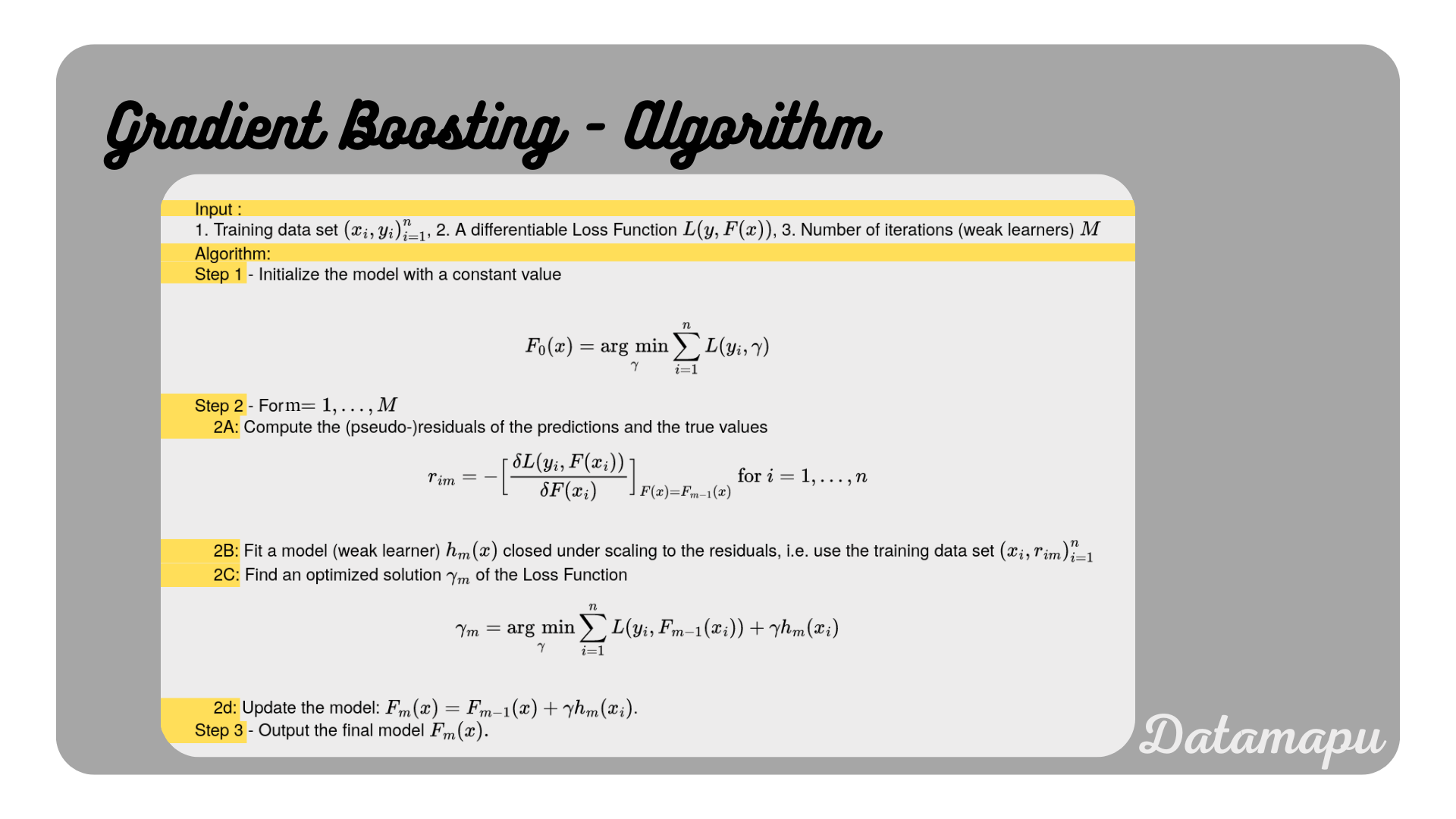“gradient boosting algorithm” Gradient Boosting Algorithm. Adapted from Wikipedia.

We will now take a look at each single step. First, we will explain the general formulation and then modify and simplify it for a regression problem with a variation of the mean squared error as the loss function and Decision Trees as underlying models. More specifically, we use as a loss for each sample $L (y_{i}, F (x_{i})) = \frac{1}{2} (y_{i} - F (x_{i}))^{2} .$ The factor $\frac{1}{2}$ is included to make the calculations easier. For a concrete example, with all the calculations included for a specific dataset, please check Gradient Boosting for Regression - Example.

Let ${(x_{i}, y_{i})}_{i = 1}^{n} = (x_{1}, y_{1}), \dots, (x_{n}, y_{n})$ be the training data, with $x = x_{0}, \dots, x_{n}$ the input features and $y = y_{0}, \dots, y_{n}$ the target values and $F (x)$ be the mapping we aim to determine to approximate the target data. Let’s start with the first step of the algorithm defined above.

Step 1 - Initialize the model with a constant value - $F_{0} (x)$ .

The initial prediction depends on the loss function ( $L$ ) we choose. Mathematically this initial prediction is defined as $F_{0} (x) = \underset{γ}{argmin} \sum_{i = 1}^{n} L (y_{i}, γ),$

where $γ$ are the predicted values. For the special case that $L$ is the loss function defined above, this can be written as

$F_{0} (x) = \underset{γ}{argmin} \frac{1}{2} \sum_{i = 1}^{n} (y_{i} - γ)^{2} .$

The expression $\underset{γ}{argmin}$ , means that we want to find the value $γ$ that minimizes the equation. To find the minimum, we need to take the derivative with respect to $γ$ and set it to zero.

$\frac{δ}{δ γ} \sum_{i = 1}^{n} L = \frac{δ}{δ γ} \sum_{i = 1}^{n} \frac{1}{2} (y_{i} - γ)^{2}$ $\frac{δ}{δ γ} \sum_{i = 1}^{n} L = - 2 \sum_{i = 1}^{n} \frac{1}{2} (y_{i} - γ)$ $\frac{δ}{δ γ} \sum_{i = 1}^{n} L = - \sum_{i = 1}^{n} y_{i} + n γ$

We set this equal to $0$ and get

$- \sum_{i = 1}^{n} y_{i} + n γ = 0$ $n γ = \sum_{i = 1}^{n} y_{i}$ $γ = \frac{1}{n} \sum_{i = 1}^{n} y_{i} = \bar{y} .$

That means, for the special loss function we considered, we get the mean of all target values as the first prediction

$F_{0} (x) = \bar{y} .$

The next steps are repeated $M$ times, with $M$ the number of weak learners or for the special case considered, Decision Trees. We can write the next steps in the form of a loop.

Step 2 - For $m = 1$ to $M$ :

2A. Compute the (pseudo-)residuals of the preditions and the true observations.

The (pseudo-)residuals $r_{i m}$ are defined as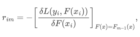
pseudo_residual

for $i = 1, \dots, n . (1 a)$

Before simplifying it for the special use case, we are considering, let’s have a closer look at this expression. The residuals $r_{i m}$ have two indices, the $m$ corresponds to the current model - remember we are building $M$ models. The second index $i$ corresponds to a data sample. That is the residuals are calculated for each sample individually. The right-hand side seems a bit overwhelming, but looking at it more closely, we can see that it is only the negative derivative of the loss function with respect to the previous prediction. In other words, it is the negative of the gradient of the Loss Function in the previous iteration. The (pseudo-)residual $r_{i m}$ thus gives the direction and the magnitude to minimize the loss function, which shows the relation to Gradient Descent.

Now, let’s see what we get, when we use the loss specified above. Using formula (1a), and $L (y_{i}, F (x_{i})) = \frac{1}{2} (y_{i} - F_{m - 1})$ simplifies the above equation to

$r_{i m} = - \frac{δ \frac{1}{2} (y_{i} - F_{m - 1})^{2}}{δ F_{m - 1}}$

$r_{i m} = (y_{i} - F_{m - 1}) (1 b)$

That is, for the special Loss $L (x_{i}, F (x_{i})) = \frac{1}{2} (y_{i} - F (x_{i}))^{2}$ , the (pseudo-)residuals $r_{i m}$ , reduce to the difference between the actual target and the predicted value, which is also known as the residual. This is also the reason, why the (pseudo-)residual has this name. If we choose a different loss function, the expression will change accordingly.

2B. Fit a model (weak learner) closed under scaling $h_{m} (x)$ to the residuals.

The next step is to train a model with the residuals as target values, that is use the data ${(x_{i}, r_{i m})}_{i = 1}^{n}$ and fit a model to it. For the special case discussed we train a Decision Tree with a restricted number of leaves or depth.

2C. Find optimized solution $γ_{m}$ for the Loss Function.

The general formulation of this step is described by solving the optimization problem

$γ_{m} = \underset{γ}{argmin} \sum_{i = 1}^{n} L (y_{i}, F_{m - 1} (x_{i}) + γ h_{m} (x_{i})), (2 a)$

where $h_{m} (x_{i})$ is the just fitted model (weak learner) at $x_{i}$ . For the case of using Decision Trees as a weak learner, $h (x_{i})$ is

$h (x_{i}) = \sum_{j = 1}^{J_{m}} b_{j m} 1_{R_{j m}} (x),$

with $J_{m}$ the number of leaves or terminal nodes of the tree, and $R_{1 m}, \dots R_{J_{m} m}$ are so-called regions. These regions refer to the terminal nodes of the Decision Tree. Because we are fitting a weak learner, that is a pruned tree, the terminal nodes will consist of several predictions. Each region relates to one constant prediction, which is the mean over all values in the according node and is denoted as $b_{j m}$ in the above equation. The notation may seem a bit complicated, but once illustrated, it should become more clear. An overview is given in the plot below.

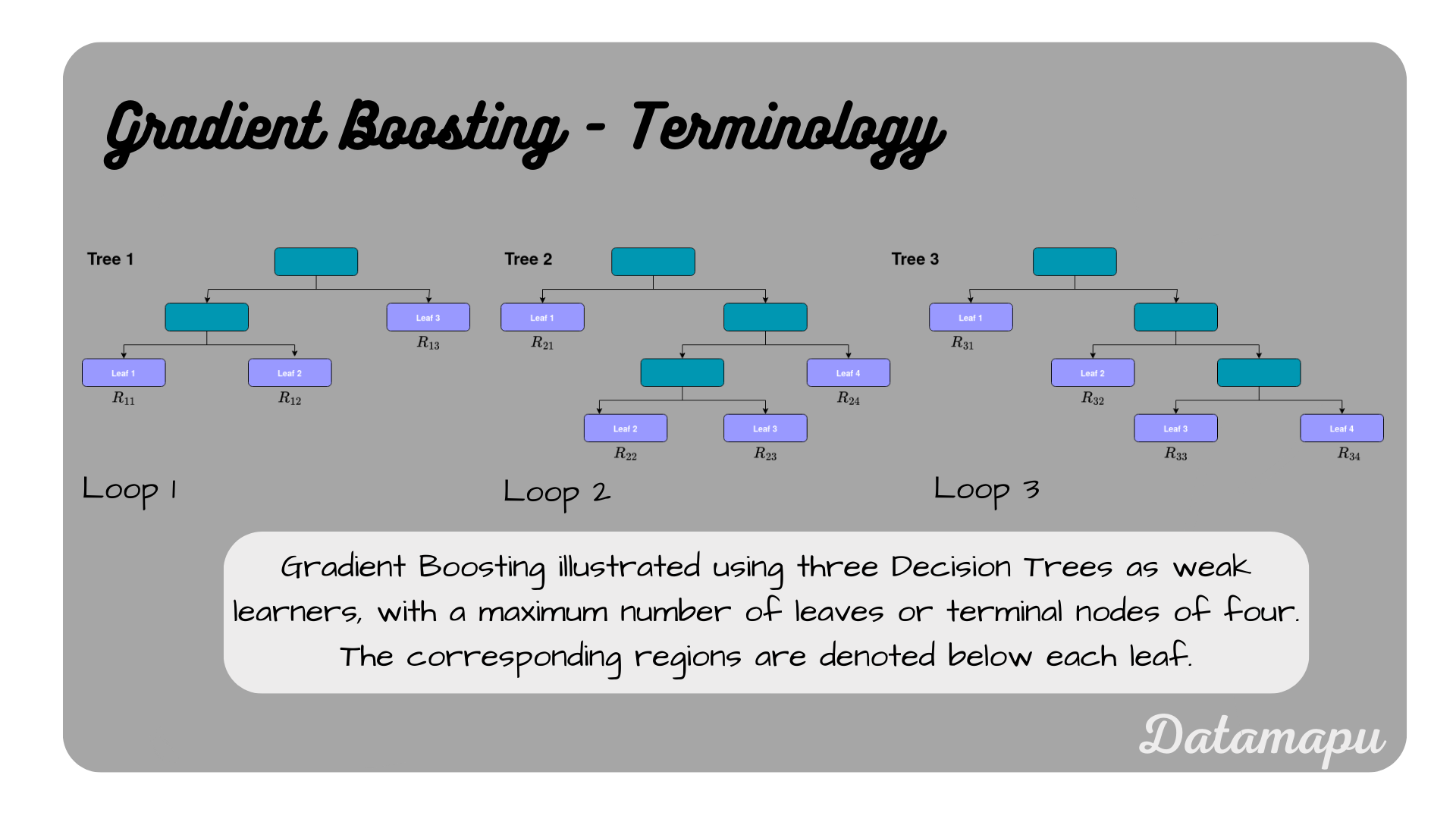Gradient Boosting Terminology Terminology for Gradient Boosting with Decision Trees.

For a Decision Tree as an underlying model, this step is a bit modified. A separate optimal value $γ_{j m}$ for each of the tree’s regions is chosen, instead of a single $γ_{m}$ for the whole tree [1, 2]. The coefficients $b_{j m}$ can be then discarded and the equation (2a) is reformulated as

$γ_{j m} = \underset{γ}{argmin} \sum_{x_{i} \in R_{j m}} L (y_{i}, F_{m - 1} (x_{i}) + γ) . (2 b)$

Note, that the sum is only taken over the elements of the region. For the special case, we are considering using the specified loss $L (y_{i}, F_{m - 1} (x_{i})) = \frac{1}{2} (y_{i} - F_{m - 1} (x_{i}))^{2}$ , (2a) reduces to

$γ_{m} = \underset{γ}{argmin} \sum_{x_{i} \in R_{j m}} \frac{1}{2} (y_{i} - (F_{m - 1} (x_{i}) + γ))^{2} .$

As explained above, this means we want to minimize the right-hand term. For that, we calculate the derivative with respect to $γ$ and set it to zero.

$\frac{δ}{δ γ} \sum_{x_{i} \in R_{j m}} \frac{1}{2} (y_{i} - F_{m - 1} (x_{i}) - γ)^{2} = 0$ $- \sum_{x_{i} \in R_{j m}} (y_{i} - F_{m - 1} (x) - γ) = 0$ $- n_{j} γ = \sum_{x_{i} \in R_{j m}} (y_{i} - F_{m - 1} (x_{i})),$

with $n_{j}$ the number of samples in the terminal node $R_{j m}$ . This leads to

$γ = \frac{1}{n_{j}} \sum_{x_{i} \in R_{j m}} r_{i m}, (2 c)$

with $r_{i m} = y_{i} - F_{m - 1} (x_{i})$ the residual. The solution that minimizes (2b) is thus the mean over all target values of the tree we constructed using the residuals as target values. That is $γ$ is nothing but the prediction we get from our tree fitted to the residuals.

2D. Update the model.

The last step in this loop is to update the model.

$F_{m} (x) = F_{m - 1} (x) + γ_{m} h_{m} (x)$

That is we use our previous model $F_{m - 1}$ and add the new predictions from the model fitted to the residuals. For the special case of Decision Trees as weak learners, this can be reformulated to

$F_{m} (x) = F_{m - 1} (x) + α \sum_{j = 1}^{J_{m}} γ_{j m} 1 (x \in R_{j m}) .$

The sum means, that we sum all values $γ_{j m}$ of the terminal node $R_{j m} .$ The factor $α$ is the learning rate, which is a hyperparameter between $0$ and $1$ that needs to be chosen. It determines the contribution of each tree and is often referred to as the scaling of the models. The learning rate $α$ is a parameter that is related to the Bias-Variance Tradeoff. A learning rate closer to $1$ usually reduces the bias, but increases the variance and vice versa. That is we choose a lower learning rate to reduce the variance and overfitting.

Step 3 - Output final model $F_{M} (x)$ .

The individual steps of the algorithm for the special case of using Decision Trees and the above specified loss is summarized below.

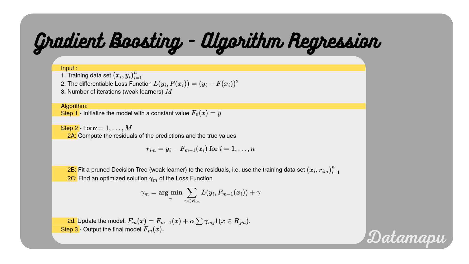Gradient Boosting for Regression Gradient Boosting Algorithm simplified for a regression task.

Gradient Boosting vs. AdaBoost (for Regression)

Another ensemble model based on boosting is AdaBoost. Although both models share the same idea of iteratively improving the model, there is a substantial difference in how the shortcomings of the developed model are defined. A comparison of both methods is summarized in the following table.

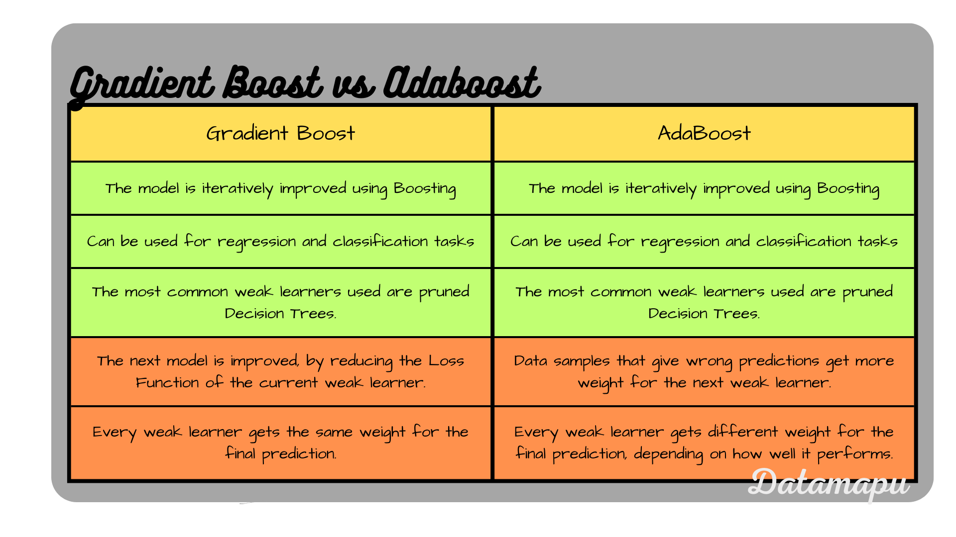Gradientboost vs AdaBoost Gradient Boost vs. AdaBoost.

Pros & Cons of Gradient Boosted Trees

Let’s now see what are the main advantages and disadvantages of Gradient Boosted Trees, as this is the most common application of Gradient Boosting.

Pros

Gradient Boosted Trees can deal with missing data and outliers in the input features, that is data preprocessing is easier.
They can are flexible considering the data type of the input features and can deal with numerical and categorical data.
Gradient Boosting can be applied for regression and classification tasks.
They are flexible considering the loss function can be used and therefore be adapted to the specified problem.

Cons

Gradient Boosting may be sensitive to outliers in the target data because every new weak learner (tree) is built on the errors (residuals) of the previous weak learner. Depending on the loss function chosen, outliers may have large residuals. With the loss used in this post, which is a variation of the Mean Squared Error outlier will have high residuals and the next weak learner will focus more on these outliers. Other Loss Functions like the Mean Absolute Error or Huber loss are less sensitive to outliers.
If the dataset is small or the model too large, i.e. too many weak learners are used Gradient Boosting may overfit.

Gradient Boosting in Python

In Python we can use the GradientBoostingRegressor from sklearn to perform a regression task with Gradient Boosting. Note, that the underlying weak learner in this method is not flexible, but is fixed to Decision Trees. Here we consider a very simple example, that contains only 10 data samples. It describes how many meters a person climbed depending on their age and whether they like height and goats. 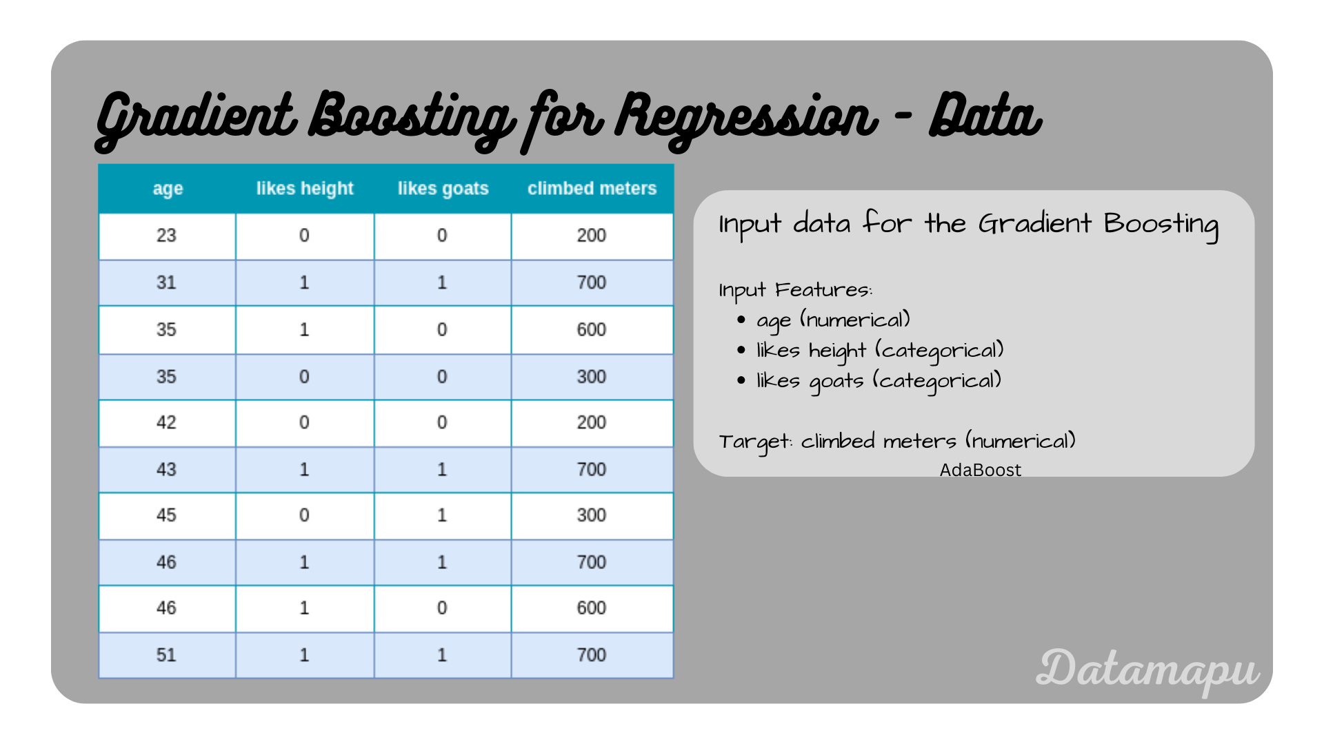gradient boosting reg data Dataset considered in this example

Let’s read the data into a Pandas dataframe.

1
2
3
4
5
6
7
8
import pandas as pd

data = {'age': [23, 31, 35, 35, 42, 43, 45, 46, 46, 51], 
        'likes goats': [0, 1, 0, 0, 0, 1, 1, 1, 0, 1], 
        'likes height': [0, 1, 1, 0, 0, 1, 0, 1, 1, 1], 
        'climbed meters': [200, 700, 600, 300, 200, 700, 300, 700, 600, 700]}

df = pd.DataFrame(data)

Now, we can fit a model to this data. There are several hyperparameters available that can be tuned to optimize the model. The most important ones are

loss: Loss Function to be optimized. It can be chosen between: ‘squared_error’, ‘absolute_error’, ‘huber’, and ‘quantile’.. ‘squared_error’ refers to the squared error for regression. ‘absolute_error’ refers to the absolute error of regression and is a robust loss function. ‘huber’ is a combination of the two. ‘quantile’ allows quantile regression (use the hyperparameter alpha to specify the quantile).
Default value: ‘squared_error’.
learning_rate: The contribution of each tree is defined by learning_rate. There is a trade-off between learning_rate and n_estimators. Values must be in the range $[0.0, inf)$ .
Default value: $0.1$ .
n_estimators: The number of boosting stages to perform or in other words the number of weak learners. Gradient Boosting is quite robust to overfitting so a large number usually results in better performance. Values must be in the range $[1, inf)$ .
Default value: 100.
max_depth: Maximum depth of the individual regression estimators. The maximum depth limits the number of nodes in the tree. If None, then nodes are expanded until all leaves are pure or until all leaves contain less than min_samples_split samples.
Default value: 3.
init: an estimator object or ‘zero’, that is used to compute the initial predictions. The init estimator has to provide a fit and a predict method.If init is set to ‘zero’, the inital predictions are set to zero.
Default value: DummyEstimator, which predicts either the average of the target value (if the loss is equal to ‘squared_error’), or a quantile for the other losses.
alpha: The alpha-quantile of the huber Loss Function and the quantile Loss Function. $a l p h a$ is only needed if loss=‘huber’ or loss=‘quantile’. Values must be in the range $(0.0, 1.0)$ .
Default value: 0.9.

A detailed list of all hyperparameters with explanations can be found in the documentation of sklearn. The pruning of the trees results from the restriction of max_depth in the default setup. We will keep all default values as they are, for this example, except the n_estimators value, which we will set to three. This is done, because our example dataset is very small. In real-world projects, n_estimators is usually much higher.

 1
 2
 3
 4
 5
 6
 7
 8
 9
10
from sklearn.ensemble import GradientBoostingRegressor

X = df[['age', 'likes goats', 'likes height']].values
y = df[['climbed meters']].values.reshape(-1,)
reg = GradientBoostingRegressor(
	n_estimators=20, 
	max_depth=3, 
    	random_state=42
	)
reg.fit(X, y)

We can now use the predict method to make predictions and calculate the score of the prediction. The score in this case is the Coefficient of Determination often abbreviated as $R^{2}$ .

1
2
y_pred = reg.predict(X)
score = reg.score(X, y)

This leads to the predictions $[246.62, 675.68, 587.84, 313.49, 249.13, 675.68, 312.33, 675.68, 587.84, 675.68]$ and a score of $0.98$ . For this simplified example, we will not go deeper, you can find a more detailed example on a larger dataset on kaggle.

Summary

In this article, we discussed the algorithm of Gradient Boosting for a regression task. Gradient Boosting is an iterative Boosting algorithm that builds a new weak learner in each step that aims to reduce the loss function. The most common setup for this is to use Decision Trees as weak learners. We used a variant of the MSE as a loss function and derived the algorithm for this case from the more general formulas. A simple example was chosen to demonstrate how to use Gradient Boosting in Python. For a more realistic example, please check this notebook on kaggle.

Introduction

The Algorithm

Step 1 - Initialize the model with a constant value - F0(x).

Step 2 - For m=1 to M: