Understanding K-Means Clustering
- 8 minutes read - 1699 wordsIntroduction
K-Means is an example of a clustering algorithm. Clustering is a fundamental concept in Machine Learning, where the goal is to group a set of objects so that objects in the same group are more similar to each other than to those in other groups. Clustering belongs to the set of unsupervised Machine Learning algorithms, that is no ground truth is needed. Among the various clustering algorithms, K-Means stands out for its simplicity and efficiency. In this blog post, we will explain the algorithm behind K-Means, and see how to implement it in Python.
Illustration of clustering.
What is K-Means Clustering? - The Algorithm
K-Means clustering is an unsupervised Machine Learning algorithm used to partition an unlabeled, unsorganised data set into k clusters, where the number k is defined in advance. Each data point is assigned to the cluster with the closest centroid, based on a predefined distance metric. The algorithm minimizes the inner-cluster variance of the data. More precisely the algorithm follows these steps:
1. Initialization: The algorithm starts by selecting k initial centroids. These can be chosen as random points from the data sets or by using more sophisticated methods like K-Means++ to improve convergence. When using the sklearn library, the initial method “k-means++” is the default method.
2. Assignment Step: For each data point, the distance to each of the centroids is calculated. Each data point is then assigned to the nearest centroid. As distance metric typically the Euclidean distance is chosen, which is also the metric used in the sklearn method. After this step k clusters are formed.
3. Update Step: The centroids are recalculated as the mean of all data points assigned to each cluster.
Repeat steps 2 and 3 iteratively until the centroids no longer change significantly or the indicated number of iterations is reached. The k clusters after reaching the convergence criterion are the final result.
Choosing the Right Number of Clusters
One of the key challenges in K-Means clustering is selecting the optimal number of clusters. Several of methods have been developed to determine the optimal number of clusters. In this post, we will only discuss the most popular ones: the Elbow Method and the Silhouette Score.
Elbow Method
The Elbow Method helps to determine the optimal number of clusters by plotting the sum of squared distances (inertia) from each point to its assigned centroid against the number of clusters. As the number of clusters increases, the inertia decreases. The point where the decrease sharply slows down (forming an “elbow”) indicates the optimal number of clusters.
This method’s popularity stems from its simplicity and visual appeal. It allows data scientists and analysts to quickly identify a suitable number of clusters by visual inspection.
Pros:
- Simple to understand and implement.
- Provides a visual indication of the optimal number of clusters.
Cons:
- The elbow point can sometimes be ambiguous or not very pronounced, making it hard to decide the optimal number of clusters.
Silhouette Method
The Silhouette Score or Silhouette Coefficient evaluates the consistency within clusters and the separation between clusters. It ranges from -1 to 1, with higher values indicating better clustering. The method is in detail described on Wikipedia. The score is calculated as follows:
1. step: For each data point $i$ in cluster $C_I$:
Calculate the mean inner-cluster distance (a): This is the average distance between the data point $i$ and all other points in the same cluster.
$$a(i) = \frac{1}{|C_I| - 1} \sum_{j\in C_I, j\neq i} d(i,j),$$
with $|C_I|$ the total number of data points in cluster $I$, and $d(i, j)$ the distance between data point $i$ and data point $j$.
Calculate the mean nearest-cluster distance (b): This is the average distance between the data point $i$ and all points in the nearest neighboring cluster.
$$b(i) = \min_{J\neq I}\frac{1}{C_J}\sum_{j\in C_J} d(i,j),$$
where $C_J$ is any other cluster than $C_I$. Since the minimum over all clusters is taken, this results in the average distance of data point $i$ and all data points in the neighboring cluster. The neighboring cluster is the next best fit cluster for data point i.
2. step: Calculate the silhouette coefficient for the data point $i$:
$$s(i) = \frac{b(i) - a(i)}{\max(a(i), b(i))}.$$
This equation holds if $|C_I| > 1$, if $|C_I| = 1$, $s(i)$ is defined as $0$.
The above equation can be rewritten as
$$ s(i) = \begin{cases} 1 - \frac{a(i)}{b(i)} & \text{if } a(i) < b(i) \newline 0 & \text{if } a(i) = b(i) \newline \frac{b(i)}{a(i)} - 1 & \text{if } a(i) > b(i) \end{cases} $$
s(i) ranges from -1 to 1:
- s(i) close to 1: The data point is well-clustered. The mean distance to the data points within the cluster is smaller than the mean distance to the data points of the neighboring cluster.
- s(i) close to 0: The data point is on or very close to the decision boundary between two neighboring clusters.
- s(i) close to -1: The data point might have been assigned to the wrong cluster. The mean distance to the data points in neighboring cluster is smaller than the mean distance to the data points within the cluster.
3. step: Calculate the mean silhouette score for all data points: The overall silhouette score for the clustering is the average silhouette coefficient for all data points.
$$S = \frac{1}{N}\sum_{i=1}^N s(i)$$
where $N$ is the total number of data points.
This method is favored because it provides a more detailed and rigorous evaluation of clustering quality, helping to ensure that the chosen number of clusters truly represents the data structure.
Pros:
- Provides a clear and quantitative measure of clustering quality.
- Works well for a variety of cluster shapes and densities.
Cons:
- Computationally more intensive than the Elbow Method, especially for large datasets.
- May not be as intuitive to interpret as the Elbow Method.
Other Methods
The Elbow method and the Silhouette Score are the most popular and the most straight forward methods. There are however several other methods, that are more complex. We are not going to explain them here, but only name a few and link to a reference.
Code Example
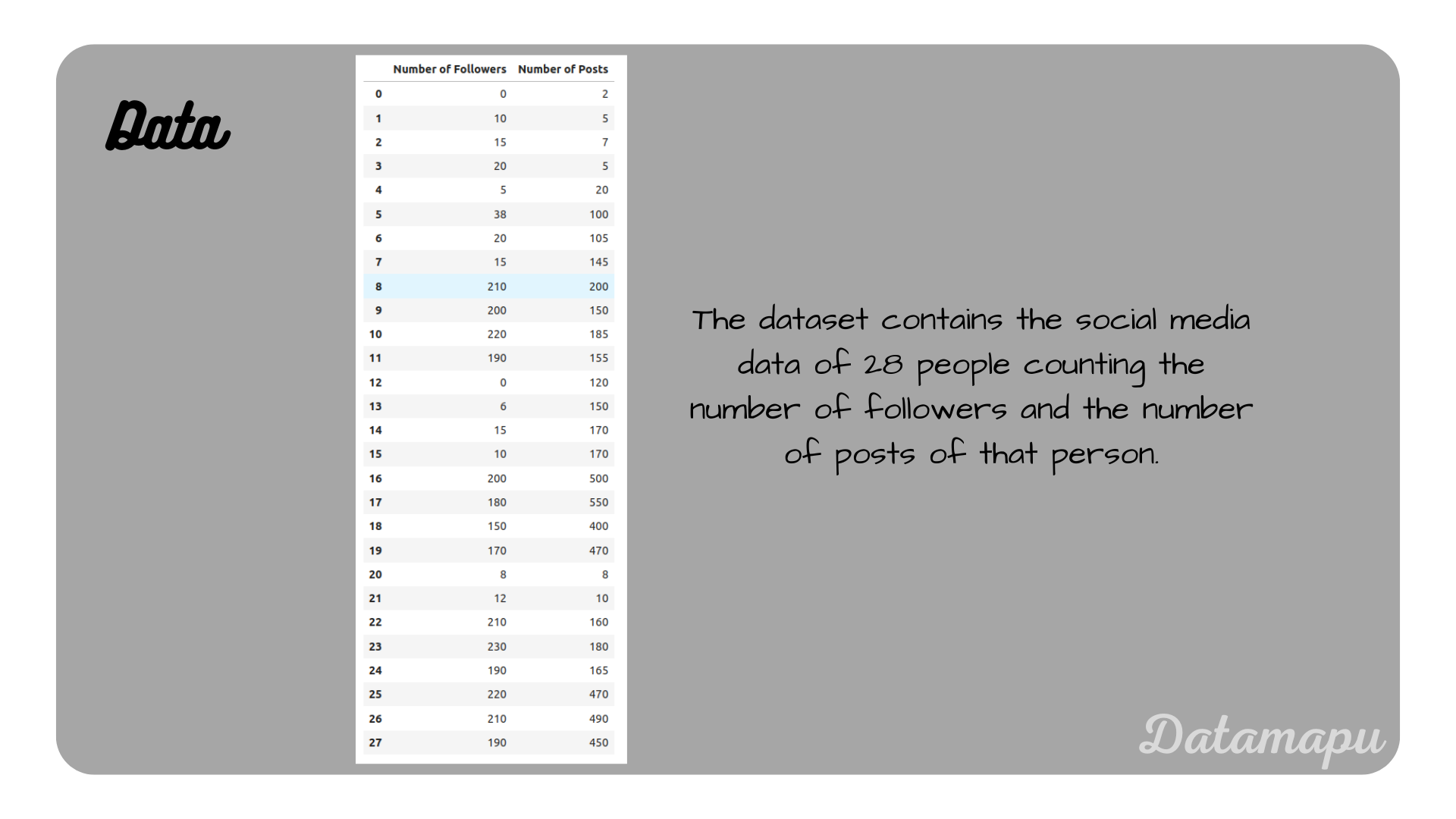
We consider a simple dataset consisting of 28 data points. The data describes the number of followers and the number of posts in a social media application for 28 persons.
 The data set used in this example.
We read this data into a Pandas dataframe and then transform it into a numpy array.
| |
We use the sklearn method KMeans with the default setup. For this demonstration, the only parameter we change is the number of clusters (n_clusters). We can, however, e.g. change the initialization method (init), the maximal number of iterations (max_iter), and the tolerance (tol) that defines the convergence of the algorithm. For all details, please refer to the documentation.
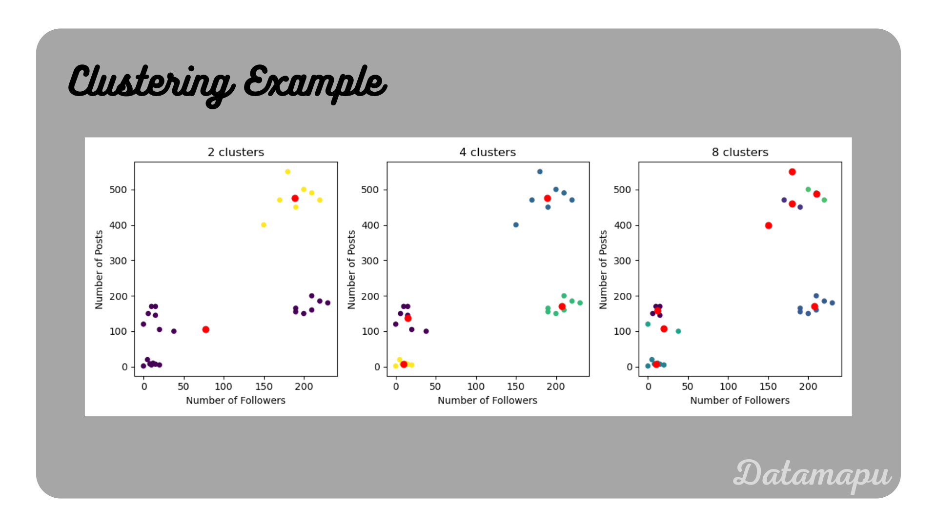
We use the defined data set to fit the KMeans method. We fit the data using $2$, $4$, and $8$ clusters and plot the results. We can then access the calculated centroids using kmeans.cluster_centers_.
| |
 Clustering the example data with $2$, $4$, and $8$ clusters.
In this simple example, we can already visually see that $4$ clusters are the correct number, but let’s use the above discussed methods to verify this.
Elbow Method
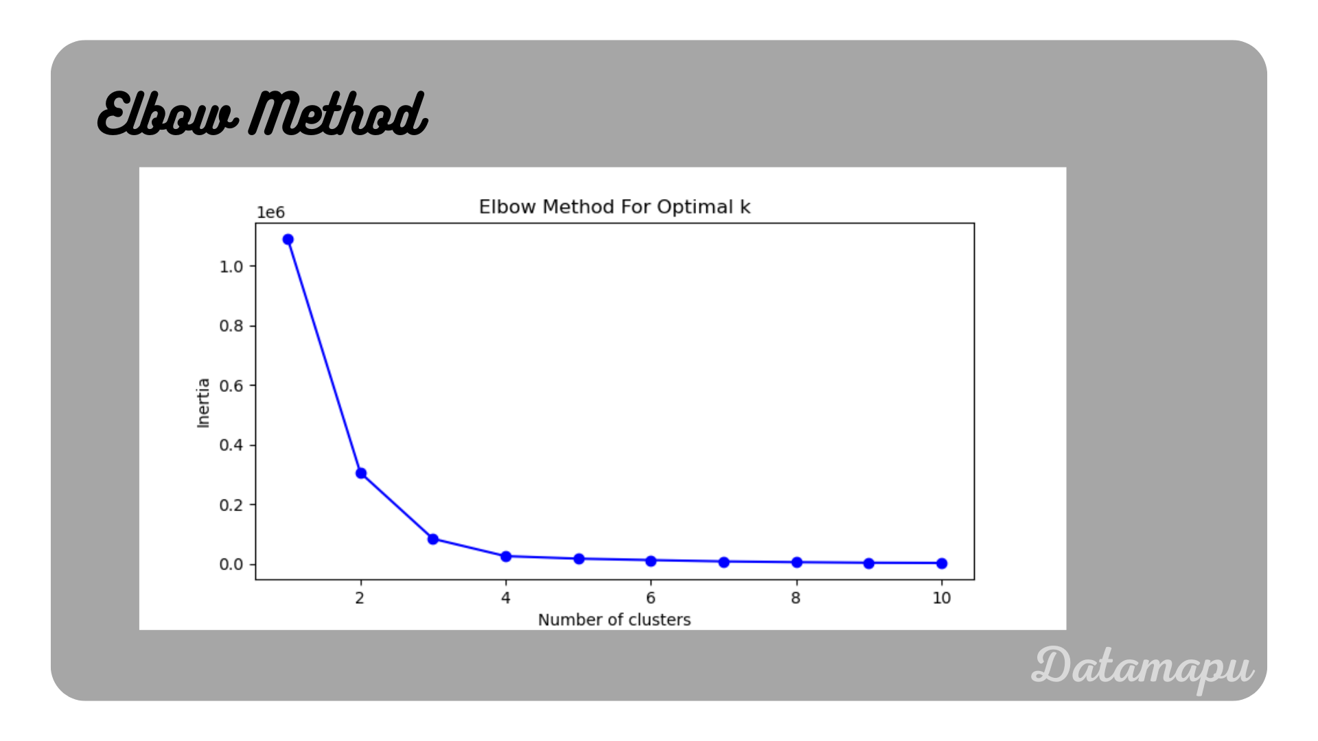
To illustrate the Elbow Method, we fit the data for an increasing number of clusters ranging from $1$ to $11$, save the inertias (sum of square distances), and plot the result.
| |
 Elbow curve for the example data.
In this plot, we see that at the beginning the curve is falling steeply and this decrease reduces strongly after reaching $4$ clusters. This indicates that this is the best number of clusters for this task.
Silhouette Score
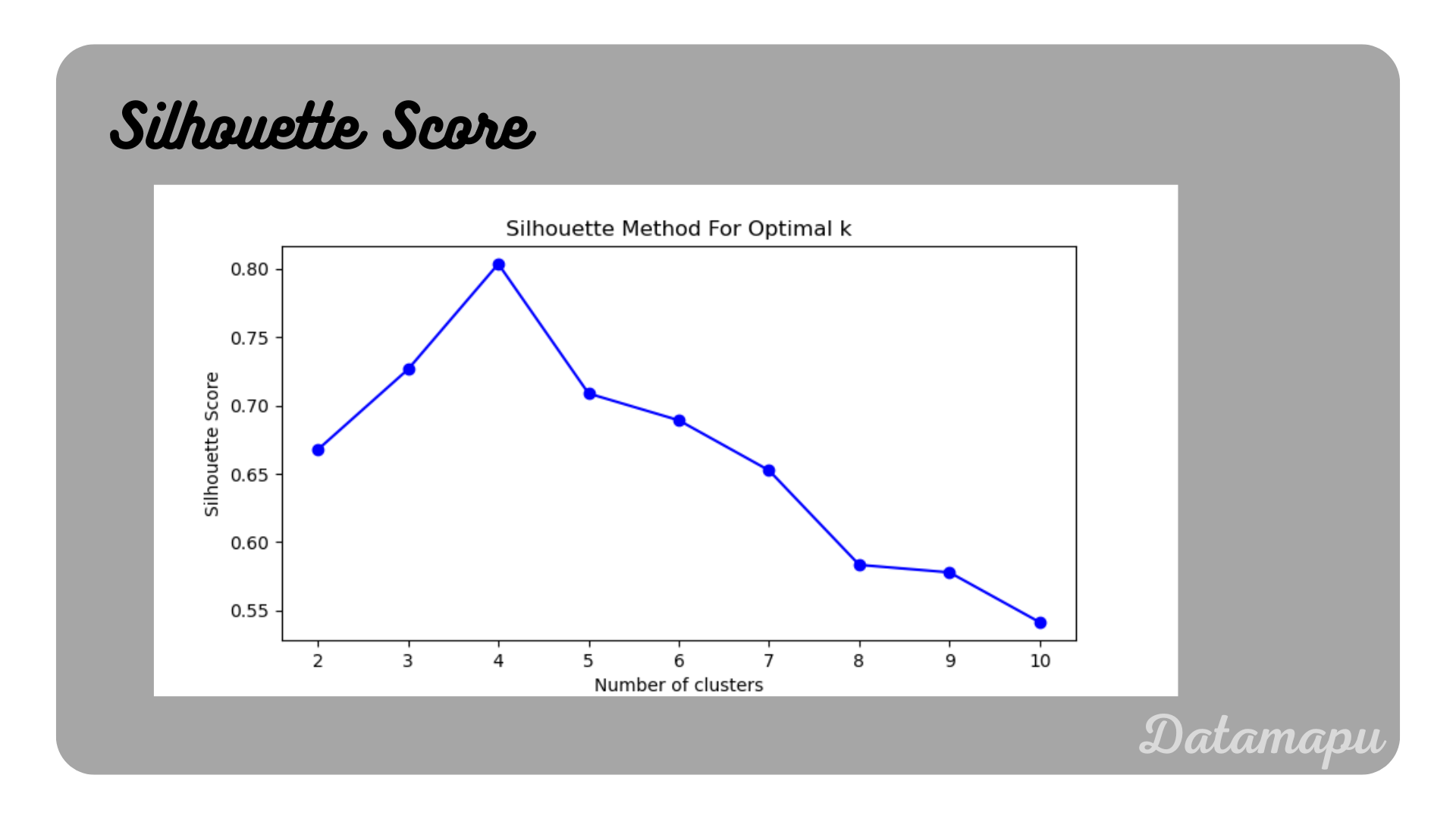
The silhouette score is also a method available in sklearn. In this case, we fit the KMeans method to a range of $2$ to $11$ clusters. For each fit, we calculate the silhouette score and plot the result.
| |
 Silhouette Score for the example data.
This plot shows a maximum for $4$ clusters, that is the silhouette score is highest for this number of clusters, which indicates the optimal number of clusters.
Summary
KMeans is an unsupervised machine learning algorithm used for clustering data into k distinct groups based on feature similarity. It works by iteratively assigning data points to the nearest cluster center and then updating the cluster centers to be the mean of the assigned points. The process continues until the cluster assignments no longer change significantly or the maximum number of iterations is reached. It is a popular algorithm due to its simplicity, efficiency with large datasets, and ease of implementation and interpretation. An example of applying KMeans to a more real-world dataset than the simplifies example above can be found on kaggle.
If this blog is useful for you, please consider supporting.
